使用逻辑函数的 COVID-19 峰值预测

如今，做出快速准确的决策至关重要，尤其是在当今世界面临 COVID-19 这样的现象时，因此，依靠当前和预测的信息对于这一过程至关重要。
在这件事上，我们应用了一个模型，在这个模型中可以观察到特定国家案例中的峰值，利用当前的统计信息，希望它可以作为在这种情况下采取行动的基础支持。为了实现这一目标，非线性回归已应用于模型，使用逻辑函数。这个过程包括：

• 数据清洗
• 选择可以以图形方式适应数据的最合适的方程，在这种情况下，逻辑函数（Sigmoid）
• 数据库规范化
• 使用“curve_fit”过程将模型拟合到我们的数据集，获得新的参考 beta。
• 模型评估

数据集是公开的，可通过以下链接在 Data.europa.eu 获得：DATASET
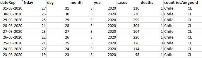
数据清洗：可用的数据最初已被标记。我们能够识别出两个未提及地理位置的国家/地区，添加了此信息，但它不会对模型产生显着影响。一个名为“n-day”的新列被添加到数据集中以显示连续天数。

代码：导入库

Python3

# import libraries
import pandas as pd
import numpy as np
import matplotlib.pyplot as plt % matplotlib inline
 
# sklearn specific function to obtain R2 calculations
from sklearn.metrics import r2_score

代码：使用数据

Python3

# Data Reading
df = pd.read_excel("C:/BaseDato / COVID-19-310302020chi.xlsx")
df.head()

输出：

代码：

Python3

# Initial Data Graphics
plt.figure(figsize =(8, 5))
 
x_data, y_data = (df["Nday"].values, df["cases"].values)
 
plt.plot(x_data, y_data, 'ro')
plt.title('Data: Cases Vs Day of infection')
plt.ylabel('Cases')
plt.xlabel('Day Number')

输出：

代码：选择模型
我们应用逻辑函数sigmoid 函数的一种特殊情况，考虑到原始曲线以缓慢增长开始，在增加之前几乎保持平坦一段时间，最终它可能会下降或以指数曲线的方式保持其增长。

逻辑函数的公式为：

Y = 1/(1+e^B1(X-B2))

代码：模型的构建

Python3

# Definition of the logistic function
def sigmoid(x, Beta_1, Beta_2):
     y = 1 / (1 + np.exp(-Beta_1*(x-Beta_2)))
     return y
 
# Choosing initial arbitrary beta parameters
beta_1 = 0.09
beta_2 = 305
 
# application of the logistic function using beta
Y_pred = sigmoid(x_data, beta_1, beta_2)
 
# point prediction
plt.plot(x_data, Y_pred * 15000000000000., label = "Model")
plt.plot(x_data, y_data, 'ro', label = "Data")
plt.title('Data Vs Model')
plt.legend(loc ='best')
plt.ylabel('Cases')
plt.xlabel('Day Number')

输出：

数据规范化：在这里，变量 x 和 y 被规范化，为它们分配 0 到 1 的范围（取决于每种情况）。因此，两者都可以同等相关地解释。
参考信息

代码：

Python3

xdata = x_data / max(x_data)
ydata = y_data / max(y_data)

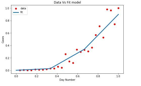
模型拟合：
目标是获得新的 B 最优参数，以根据我们的数据调整模型。我们使用“curve_fit”，它使用非线性最小二乘来拟合 sigmoid函数。 “弹出”我们优化的参数。

代码：输入

Python3

from scipy.optimize import curve_fit
popt, pcov = curve_fit(sigmoid, xdata, data)
 
# imprimir los parámetros finales
print(" beta_1 = % f, beta_2 = % f" % (popt[0], popt[1]))

输出：

beta_1 = 9.833364, beta_2 = 0.777140

代码：新的 Beta 值应用于模型

Python3

x = np.linspace(0, 40, 4)
x = x / max(x)
 
plt.figure(figsize = (8, 5))
 
y = sigmoid(x, *popt)
 
plt.plot(xdata, ydata, 'ro', label ='data')
plt.plot(x, y, linewidth = 3.0, label ='fit')
plt.title("Data Vs Fit model")
plt.legend(loc ='best')
plt.ylabel('Cases')
plt.xlabel('Day Number')
plt.show()

模型评估：模型已准备好进行评估。数据在 80:20 拆分，分别用于训练和测试。将数据应用于获得相应统计手段的模型，以评估结果数据与回归线的距离。

代码：输入

Python3

# Model accuracy calculation
# Splitting training and testing data
 
L = np.random.rand(len(df)) < 0.8 # 80 % training data
train_x = xdata[L]
test_x = xdata[~L]
train_y = ydata[L]
test_y = ydata[~L]
 
# Construction of the model
popt, pcov = curve_fit(sigmoid, train_x, train_y)
 
# Predicting using testing model
y_predic = sigmoid(test_x, *popt)
 
# Evaluation
print("Mean Absolute Error: %.2f" % np.mean(np.absolute(y_predic - test_y)))
print("Mean Square Error (MSE): %.2f" % np.mean(( test_y - y_predic)**2))
print("R2-score: %.2f" % r2_score(y_predic, test_y))

输出：

Mean Absolute Error: 0.06
Mean Square Error (MSE): 0.01
R2-score: 0.93