在Python中处理地理空间数据

空间数据，也称为地理空间数据、GIS 数据或地理数据，是一种数值数据，用于定义物理对象的地理位置，例如建筑物、街道、城镇、城市、国家或其他物理对象，使用地理坐标系。您不仅可以使用空间数据确定对象的位置，还可以确定其长度、大小、面积和形状。

要在Python中处理地理空间数据，我们需要GeoPandas & GeoPlot 库

GeoPandas 是一个开源项目，使在Python中处理地理空间数据更容易。 GeoPandas 扩展了 Pandas 使用的数据类型，以允许对几何类型进行空间操作。几何运算被匀称地执行。 Geopandas 进一步依赖 fiona 进行文件访问和 matplotlib 进行绘图。 GeoPandas 依赖于它在大型地理空间、开源库堆栈（GEOS、GDAL 和 PROJ）上的空间功能。有关更多详细信息，请参阅下面的依赖项部分。

所需的依赖项：

• 麻木的
• 熊猫（版本 0.24 或更高版本）
• 匀称（与 GEOS 的接口）
• fiona（与GDAL的接口）
• pyproj（PROJ 接口；版本 2.2.0 或更高版本）

此外，可选的依赖项是：

• rtree（可选；用于提高性能和覆盖操作所需的空间索引；libspatialindex 的接口）
• psycopg2（可选；用于 PostGIS 连接）
• GeoAlchemy2（可选；用于写入 PostGIS）
• geopy（可选；对于绘图，这些附加用于地理编码）

可以使用包：

• matplotlib (>= 2.2.0)
• 地图分类 (>= 2.2.0)

Geoplot 是一个地理空间数据可视化库，适用于希望快速完成工作的数据科学家和地理空间分析师。下面我们将介绍 Geoplot 的基础知识并探索它是如何应用的。 Geoplot 仅适用于Python 3.6+ 版本。

注意：请安装所有依赖项和模块以使给定代码正常运行。

安装

• 安装可以通过 Anaconda 完成：

句法：

conda install geopandas
conda install geoplot

• conda-forge 是一项社区成果，为各种软件提供 conda 包。除了 Anaconda 提供的“默认”频道之外，它还为 conda 提供了 conda-forge 软件包频道，从中可以安装软件包。 GeoPandas 及其所有依赖项在 conda-forge 频道上可用，并且可以安装为：

句法：

conda install --channel conda-forge geopandas
conda install geoplot -c conda-forge

• 如果可以安装所有依赖项，也可以使用 pip 安装 GeoPandas：

句法：

pip install geopandas
pip install geoplot

• 您可以通过克隆 GitHub 存储库并使用 pip 从本地目录安装来安装最新的开发版本：

句法：

git clone https://github.com/geopandas/geopandas.git
cd geopandas
pip install

• 也可以直接从 GitHub 存储库安装最新的开发版本：

句法：

pip install git+git://github.com/geopandas/geopandas.git

安装软件包及其依赖项后，打开像 spyder 这样的Python编辑器。在开始编写代码之前，我们需要下载一些 shapefile（扩展名为 .shp）。您可以从这里的“免费空间数据”下下载国家级数据以及全球级数据。要获取教程中使用的 shapefile，请单击此处。

读取形状文件

首先，我们将导入 geopandas 库，然后使用变量“world_data”读取我们的 shapefile。 Geopandas 可以使用以下命令读取几乎任何基于矢量的空间数据格式，包括 ESRI shapefile、GeoJSON 文件等：

Syntax: geopandas.read_file()

Parameters

• filename: str, path object, or file-like object. Either the absolute or relative path to the file or URL to be opened or any object with a read() method (such as an open file or StringIO)
• bbox: tuple | GeoDataFrame or GeoSeries | shapely Geometry, default None. Filter features by given bounding box, GeoSeries, GeoDataFrame or a shapely geometry. CRS mis-matches are resolved if given a GeoSeries or GeoDataFrame. Cannot be used with mask.
• mask: dict | GeoDataFrame or GeoSeries | shapely Geometry, default None. Filter for features that intersect with the given dict-like geojson geometry, GeoSeries, GeoDataFrame or shapely geometry. CRS mis-matches are resolved if given a GeoSeries or GeoDataFrame. Cannot be used with bbox.
• rows: int or slice, default None. Load in specific rows by passing an integer (first n rows) or a slice() object.
• **kwargs : Keyword args to be passed to the open or BytesCollection method in the fiona library when opening the file. For more information on possible keywords, type: import fiona; help(fiona.open)

例子：

Python3

import geopandas as gpd
  
# Reading the world shapefile
world_data = gpd.read_file(r'world.shp')
  
world_data

输出：

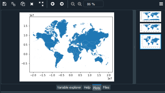
绘图

如果您想检查您使用的是哪种类型的数据，请转到控制台并输入“type(world_data)”，它告诉您这不是熊猫数据，而是地理熊猫地理数据。接下来，我们将使用 plot() 方法绘制这些 GeoDataFrames。

Syntax: GeoDataFrame.plot()

例子：

蟒蛇3

import geopandas as gpd
  
# Reading the world shapefile
world_data = gpd.read_file(r'world.shp')
  
world_data.plot()

输出：

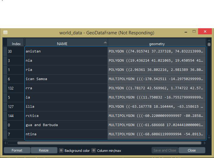
选择列

如果我们看到“world_data” GeoDataFrame 中显示了许多列（Geoseries），您可以通过以下方式选择特定的 Geoseries：

句法：

data[[‘attribute 1’, ‘attribute 2’]]

例子：

蟒蛇3

import geopandas as gpd
  
# Reading the world shapefile
world_data = gpd.read_file(r'world.shp')
  
world_data = world_data[['NAME', 'geometry']]

输出：

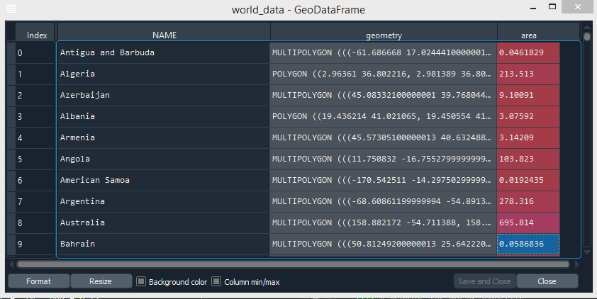
计算面积

我们可以通过创建一个新列“area”并使用 area 属性来使用 geopandas 计算每个国家的面积。

句法：

GeoSeries.area

返回一个系列，其中包含以 CRS 为单位表示的 GeoSeries 中每个几何图形的面积。

例子：

蟒蛇3

import geopandas as gpd
  
# Reading the world shapefile
world_data = gpd.read_file(r'world.shp')
  
world_data = world_data[['NAME', 'geometry']]
  
# Calculating the area of each country
world_data['area'] = world_data.area

输出：

移除一个大陆

我们可以从 Geoseries 中删除特定元素。在这里，我们将从“名称”地质系列中删除名为“南极洲”的大陆。

句法：

data[data[‘attribute’] != ‘element’]

例子：

蟒蛇3

import geopandas as gpd
  
# Reading the world shapefile
world_data = gpd.read_file(r'world.shp')
  
world_data = world_data[['NAME', 'geometry']]
  
# Calculating the area of each country
world_data['area'] = world_data.area
  
# Removing Antarctica from GeoPandas GeoDataframe
world_data = world_data[world_data['NAME'] != 'Antarctica']
world_data.plot()

输出：

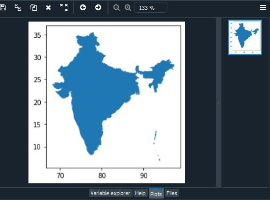
可视化特定国家

我们可以通过选择它来可视化/绘制特定国家/地区。在下面的示例中，我们从“NAME”列中选择“India”。

句法：

data[data.attribute==”element”].plot()

例子：

蟒蛇3

import geopandas as gpd
import matplotlib.pyplot as plt 
from mpl_toolkits.axes_grid1 import make_axes_locatable 
  
# Reading the world shapefile 
world_data = gpd.read_file(r'world.shp')
world_data = world_data[['NAME', 'geometry']]
  
# Calculating the area of each country 
world_data['area'] = world_data.area
  
# Removing Antarctica from GeoPandas GeoDataframe
world_data = world_data[world_data['NAME'] != 'Antarctica']
world_data[world_data.NAME=="India"].plot()

输出：

坐标参考系

我们可以使用 Geopandas CRS（即坐标参考系统）检查我们当前的坐标系统。此外，我们可以将其更改为投影协调系统。坐标参考系统 (CRS) 表示为 pyproj.CRS 对象。我们可以使用以下语法检查当前的 CRS。

句法：

GeoDataFrame.crs

to_crs() 方法将几何图形转换为新的坐标参考系统。将活动几何列中的所有几何转换为不同的坐标参考系统。必须设置当前 GeoSeries 上的 CRS 属性。可以为输出指定 CRS 或 epsg。此方法将转换所有对象中的所有点。它没有概念或投影整个几何图形。假定所有线段连接点都在当前投影中排列，而不是测地线。跨越日期变更线（或其他投影边界）的物体将有不良行为。

Syntax: GeoDataFrame.to_crs(crs=None, epsg=None, inplace=False)

Parameters

• crs: pyproj.CRS, optional if epsg is specified. The value can be anything accepted by pyproj.CRS.from_user_input(), such as an authority string (eg “EPSG:4326”) or a WKT string.
• epsg: int, optional if crs is specified. EPSG code specifying output projection.
• inplace: bool, optional, default: False. Whether to return a new GeoDataFrame or do the transformation in place.

例子：

蟒蛇3

import geopandas as gpd
  
# Reading the world shapefile
world_data = gpd.read_file(r'world.shp')
  
world_data = world_data[['NAME', 'geometry']]
  
# Calculating the area of each country
world_data['area'] = world_data.area
  
# Removing Antarctica from GeoPandas GeoDataframe
world_data = world_data[world_data['NAME'] != 'Antarctica']
  
# Changing the projection
current_crs = world_data.crs
world_data.to_crs(epsg=3857, inplace=True)
  
world.plot()

输出：

使用颜色映射 (cmap)

我们可以使用 head 列和 cmap 为世界上的每个国家/地区着色。在控制台中找出头列类型“world_data.head()”。我们可以选择 matplotlib 中可用的不同颜色图（cmap）。在以下代码中，我们使用 plot() 参数列和 cmap 为国家/地区着色。

例子：

蟒蛇3

import geopandas as gpd
  
# Reading the world shapefile
world_data = gpd.read_file(r'world.shp')
  
world_data = world_data[['NAME', 'geometry']]
  
# Calculating the area of each country
world_data['area'] = world_data.area
  
# Removing Antarctica from GeoPandas GeoDataframe
world_data = world_data[world_data['NAME'] != 'Antarctica']
  
# Changing the projection
current_crs = world_data.crs
world_data.to_crs(epsg=3857, inplace=True)
  
world_data.plot(column='NAME', cmap='hsv')

输出：

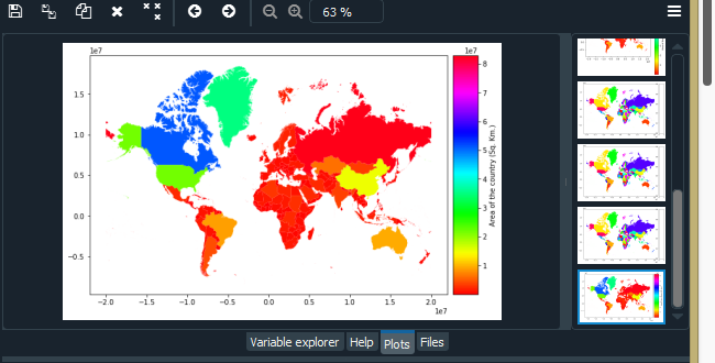
添加图例

接下来，我们将通过将面积除以 10^6 即 (1000000) 来转换以平方公里为单位的面积。输出可以在变量资源管理器中的“world_data”变量中看到。

我们可以使用 plot() 参数向我们的世界地图添加图例和标签

• 图例： bool（默认为 False）。绘制传奇。如果未指定列或指定颜色，则忽略。
• Legend_kwds：字典（默认无）。传递给 matplotlib.pyplot.legend() 或 matplotlib.pyplot.colorbar() 的关键字参数。指定方案时其他接受的关键字：
  • fmt：字符串。图例中类的 bin 边缘的格式规范。例如，没有小数：{“fmt”：“{:.0f}”}。
  • 标签：类似列表。用于覆盖自动生成标签的图例标签列表。需要具有与类数 (k) 相同数量的元素。
  • 间隔：布尔值（默认为 False）。从地图分类图例中控制括号的选项。如果为 True，则图例中会显示开/闭区间括号。

例子：

蟒蛇3

import geopandas as gpd
  
# Reading the world shapefile
world_data = gpd.read_file(r'world.shp')
  
world_data = world_data[['NAME', 'geometry']]
  
# Calculating the area of each country
world_data['area'] = world_data.area
  
# Removing Antarctica from GeoPandas GeoDataframe
world_data = world_data[world_data['NAME'] != 'Antarctica']
world_data.plot()
  
# Changing the projection
current_crs = world_data.crs
world_data.to_crs(epsg=3857, inplace=True)
world_data.plot(column='NAME', cmap='hsv')
  
# Re-calculate the areas in Sq. Km.
world_data['area'] = world_data.area/1000000
  
# Adding a legend
world_data.plot(column='area', cmap='hsv', legend=True,
                legend_kwds={'label': "Area of the country (Sq. Km.)"}, 
                figsize=(7, 7))

输出：

调整图例大小

我们还可以使用 plot() 的 ax 和 cax 参数调整图例的大小。

• 斧头： matplotlib.pyplot。艺术家（默认无）。在其上绘制绘图的轴。
• cax： matplotlib.pyplot 艺术家（默认为无）。在彩色地图的情况下绘制图例的轴。

为此，我们需要 matplotlib 库。

axis_divider.make_axes_locatable函数采用现有轴，将其添加到新的 AxesDivider，并返回 AxesDivider。然后可以使用 AxesDivider 的 append_axes 方法在原始轴的给定侧（“顶部”、“右侧”、“底部”或“左侧”）创建新轴。要在给定位置创建与主轴具有相同高度（或宽度）的轴 -

句法：

append_axes(self, position, size, pad=None, add_to_figure=True, **kwargs)

position 可以取任何值：“left”、“right”、“bottom”或“top”。

size 和 pad 应该是 axes_grid.axes_size 兼容的。

例子：

蟒蛇3

import geopandas as gpd
import matplotlib.pyplot as plt
from mpl_toolkits.axes_grid1 import make_axes_locatable
  
# Reading the world shapefile
world_data = gpd.read_file(r'world.shp')
  
world_data = world_data[['NAME', 'geometry']]
  
# Calculating the area of each country
world_data['area'] = world_data.area
  
# Removing Antarctica from GeoPandas GeoDataframe
world_data = world_data[world_data['NAME'] != 'Antarctica']
world_data.plot()
  
# Changing the projection
current_crs = world_data.crs
world_data.to_crs(epsg=3857, inplace=True)
world_data.plot(column='NAME', cmap='hsv')
  
# Re-calculate the areas in Sq. Km.
world_data['area'] = world_data.area/1000000
  
# Adding a legend
world_data.plot(column='area', cmap='hsv', legend=True,
                legend_kwds={'label': "Area of the country (Sq. Km.)"}, 
                figsize=(7, 7))
  
# Resizing the legend
fig, ax = plt.subplots(figsize=(10, 10))
divider = make_axes_locatable(ax)
  
cax = divider.append_axes("right", size="7%", pad=0.1)
world_data.plot(column='area', cmap='hsv', legend=True,
                legend_kwds={'label': "Area of the country (Sq. Km.)"},
                ax=ax, cax=cax)

输出：

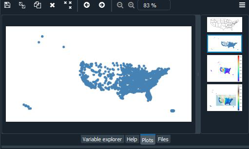
使用 Geoplot 库的 Polyplot 和 Pointplot

首先，我们将导入 Geoplot 库。接下来，我们将加载 geoplot 中存在的示例数据集之一（geojson 文件）。在下面的示例中，我们将使用“world”、“contiguous_usa”、“usa_cities”、“melbourne”和“melbourne_schools”数据集。下面提到了 geoplot 中存在的数据集列表：

• usa_cities
• contiguous_usa
• nyc_collision_factors
• nyc_boroughs
• 纽约人口普查
• 肥胖状态
• la_flights
• dc_roads
• nyc_map_pluto_sample
• nyc_collisions_sample
• boston_zip_codes
• boston_airbnb_listings
• napoleon_troop_movements
• nyc_fatal_collisions
• nyc_injurious_collisions
• nyc_police_precincts
• nyc_parking_tickets
• 世界
• 墨尔本
• 墨尔本学校
• 旧金山
• san_francisco_street_trees_sample
• california_congressional_districts

我们可以通过编辑 datasets.py 文件来添加我们自己的数据集。单击此处获取一些免费示例数据集。

• 如果您有多边形数据，则可以使用 geoplot polyplot 绘制该数据。
• 如果您的数据由一堆点组成，则可以使用 pointplot 显示这些点。

句法 ：

geoplot.datasets.get_path(str)

绘图语法：

geoplot.polyplot(var)
geoplot.pointplot(var)

例子：

蟒蛇3

import geoplot as gplt
import geopandas as gpd
  
# Reading the world shapefile
path = gplt.datasets.get_path("world")
world = gpd.read_file(path)
gplt.polyplot(world)
  
path = gplt.datasets.get_path("contiguous_usa")
contiguous_usa = gpd.read_file(path)
gplt.polyplot(contiguous_usa)
  
path = gplt.datasets.get_path("usa_cities")
usa_cities = gpd.read_file(path)
gplt.pointplot(usa_cities)
  
path = gplt.datasets.get_path("melbourne")
melbourne = gpd.read_file(path)
gplt.polyplot(melbourne)
  
path = gplt.datasets.get_path("melbourne_schools")
melbourne_schools = gpd.read_file(path)
gplt.pointplot(melbourne_schools)

世界数据集：

美国数据集：

美国城市数据集：

墨尔本数据集：

墨尔本学校数据集：

我们可以使用重叠绘制来组合这两个图。 Overplotting 是将几个不同的图相互叠加的行为，有助于为我们的图提供额外的上下文：

例子：

蟒蛇3

import geoplot as gplt
import geopandas as gpd
  
# Reading the world shapefile 
path = gplt.datasets.get_path("usa_cities")
usa_cities = gpd.read_file(path)
  
path = gplt.datasets.get_path("contiguous_usa")
contiguous_usa = gpd.read_file(path)
  
path = gplt.datasets.get_path("melbourne")
melbourne = gpd.read_file(path)
  
path = gplt.datasets.get_path("melbourne_schools")
melbourne_schools = gpd.read_file(path)
  
ax = gplt.polyplot(contiguous_usa)
gplt.pointplot(usa_cities, ax=ax)
  
ax = gplt.polyplot(melbourne)
gplt.pointplot(melbourne_schools, ax=ax)

输出：

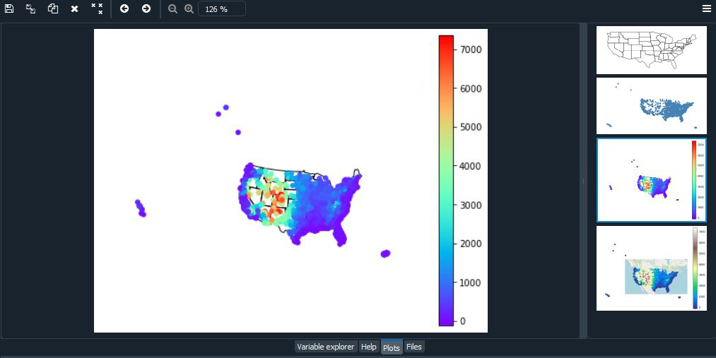
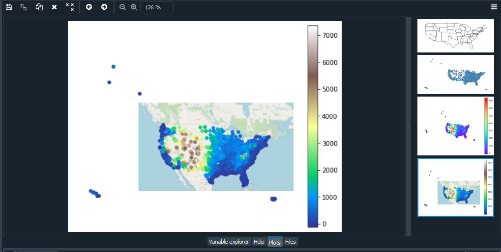
您可能已经注意到，这张美国地图看起来很奇怪。因为地球是一个球体，所以很难用二维来描绘它。因此，每当我们从球体中取出数据并将其放置在地图上时，我们都会使用某种类型的投影或将球体展平的方法。当您在没有投影或“全权委托”的情况下绘制数据时，您的地图将被扭曲。我们可以通过选择一种投影方法来“纠正”失真。这里我们将使用 Albers 等面积投影和 WebMercator 投影。

除此之外，我们还将添加一些其他参数，例如色调、图例、cmap 和方案。

• 色调参数将颜色图应用于数据列。
• 图例参数切换图例。
• 使用 matplotlib 的 cmap 更改颜色图。
• 对于分类颜色图，请使用方案。

例子：

蟒蛇3

import geoplot as gplt
import geopandas as gpd
import geoplot.crs as gcrs
  
# Reading the world shapefile 
path = gplt.datasets.get_path("contiguous_usa")
contiguous_usa = gpd.read_file(path)
  
path = gplt.datasets.get_path("usa_cities")
usa_cities = gpd.read_file(path)
  
ax = gplt.polyplot(contiguous_usa, projection=gcrs.AlbersEqualArea())
gplt.pointplot(usa_cities, ax=ax, hue="ELEV_IN_FT",cmap='rainbow', 
               legend=True)
  
ax = gplt.webmap(contiguous_usa, projection=gcrs.WebMercator())
gplt.pointplot(usa_cities, ax=ax, hue='ELEV_IN_FT', cmap='terrain', 
               legend=True)

输出：

Geoplot中的等值线

choropleth 获取在某个有意义的多边形级别（例如人口普查区、州、国家或大洲）上聚合的数据，并使用颜色将其显示给读者。它是一种众所周知的绘图类型，它可能是空间绘图类型中最通用和最广为人知的。基本的等值线需要多边形几何图形和色调变量。使用 matplotlib 的 cmap 更改颜色图。图例参数切换图例。

句法：

geoplot.choropleth(var)

例子：

蟒蛇3

import geoplot as gplt
import geopandas as gpd
import geoplot.crs as gcrs
  
# Reading the world shapefile 
boroughs = gpd.read_file(gplt.datasets.get_path('nyc_boroughs'))
  
gplt.choropleth(boroughs, hue='Shape_Area', 
                projection=gcrs.AlbersEqualArea(), 
                cmap='RdPu', legend=True)

输出：

要将关键字参数传递给图例，请使用 legend_kwargs 参数。要指定分类颜色图，请使用方案。使用legend_labels 和legend_values 自定义出现在图例中的标签和值。在这里，我们将使用 mapclassify，它是一个用于 Choropleth 地图分类的开源Python库。要安装 mapclassify 使用：

• mapclassify 可通过 conda-forge 频道在 conda 中使用：

句法：

conda install -c conda-forge mapclassify

• mapclassify 也可在Python包索引中找到：

句法：

pip install -U mapclassify

例子：

蟒蛇3

import geoplot as gplt
import geopandas as gpd
import geoplot.crs as gcrs
import mapclassify as mc
  
# Reading the world shapefile 
contiguous_usa = gpd.read_file(gplt.datasets.get_path('contiguous_usa'))
  
scheme = mc.FisherJenks(contiguous_usa['population'], k=5)
  
gplt.choropleth(
    contiguous_usa, hue='population', projection=gcrs.AlbersEqualArea(),
    edgecolor='white', linewidth=1,
    cmap='Reds', legend=True, legend_kwargs={'loc': 'lower left'},
    scheme=scheme,   legend_labels=[
        '<3 million', '3-6.7 million', '6.7-12.8 million',
        '12.8-25 million', '25-37 million'
    ]
)

输出：

Geoplot 中的 KDE 绘图

核密度估计是一种在不使用参数的情况下以非参数方式估计一组点观察的分布函数的技术。 KDE 是一种用于检查数据分布的流行方法；在此图中，该技术应用于地理空间情况。基本的 KDEplot 将逐点数据作为输入。

句法：

geoplot.kdeplot(var)

例子：

蟒蛇3

import geoplot as gplt
import geopandas as gpd
import geoplot.crs as gcrs
  
# Reading the world shapefile 
boroughs = gpd.read_file(gplt.datasets.get_path('nyc_boroughs'))
  
collisions = gpd.read_file(gplt.datasets.get_path('nyc_collision_factors'))
  
ax = gplt.polyplot(boroughs, projection=gcrs.AlbersEqualArea())
  
gplt.kdeplot(collisions, ax=ax)

输出：

Geoplot中的Sankey

桑基图描绘了通过网络的信息流。它可用于显示流经系统的数据量级。例如，该图将桑基图置于地理空间上下文中，有助于监控道路网络上的交通负载或机场之间的旅行量。一个基本的 Sankey 需要一个由 LineString 或 MultiPoint 几何组成的 GeoDataFrame。色调为地图添加颜色渐变。使用 matplotlib 的 cmap 来控制颜色图。对于分类颜色图，请指定方案。图例切换图例。这里我们使用 Mollweide 投影

句法;

geoplot.sankey(var)

例子：

蟒蛇3

import geoplot as gplt
import geopandas as gpd
import geoplot.crs as gcrs
import mapclassify as mc
  
# Reading the world shapefile 
la_flights = gpd.read_file(gplt.datasets.get_path('la_flights'))
world = gpd.read_file(gplt.datasets.get_path('world'))
scheme = mc.Quantiles(la_flights['Passengers'], k=5)
  
ax = gplt.sankey(la_flights, projection=gcrs.Mollweide(), 
                 scale='Passengers', hue='Passengers', 
                 scheme=scheme, cmap='Oranges', legend=True)
  
gplt.polyplot(world, ax=ax, facecolor='lightgray', edgecolor='white')
ax.set_global(); ax.outline_patch.set_visible(True)

输出：