在 R 编程中构建简单的神经网络
神经网络一词是指本质上是有机的或人工的神经元系统。在人工智能参考中,神经网络是一组算法,旨在识别类似于人脑的模式。他们通过一种机器感知、标记或聚类原始输入来解释感官数据。识别是数字的,它存储在向量中,所有现实世界的数据,无论是图像、声音、文本还是时间序列,都必须转换成向量。神经网络可以被描绘成一个系统,它由许多高度互连的节点(称为“神经元”)组成,这些节点按层组织,使用对外部输入的动态响应来处理信息。在了解神经网络的工作原理和架构之前,让我们尝试了解人工神经元到底是什么。
人工神经元
感知器:感知器是一种人工神经元,由科学家 Frank Rosenbalt 在 1950 年代和 1960 年代开发,其灵感来自 Warren McCulloch 和 Walter Pitts 的早期工作。那么,感知器是如何工作的呢?感知器接受多个二进制输出 x 1 、 x 2 、……,并产生单个二进制输出。
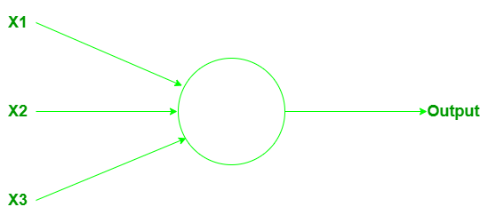
它可以有更多或更少的输入。计算/计算输出权重起着重要作用。权重 w 1 , w 2 , .... 是实数,表示各个输入对输出的重要性。神经元的输出(o 或 1)完全取决于阈值,并根据函数计算:

这里t 0是阈值。它是一个实数,是神经元的参数。这就是基本的数学模型。感知器是一种通过权衡证据做出决定的设备。通过改变权重和阈值,我们可以获得不同的决策模型。
Sigmoid 神经元: Sigmoid 神经元非常接近感知器,但经过修改后,它们的权重和偏差的微小变化只会导致其输出的微小变化。它将允许 sigmoid 神经元网络更有效地学习。就像感知器一样,sigmoid 神经元有输入,x 1 ,x 2 ,……。但是,这些输入不仅可以是 0 或 1,还可以是 0 到 1 之间的任何值。因此,例如,0.567... 是 sigmoid 神经元的有效输入。一个 sigmoid 神经元还具有每个输入的权重 w 1 、 w 2 、...,以及一个总体偏差 b。但输出不是 0 或 1。而是 σ(wx + b),其中 σ 称为 sigmoid函数:

输入为 x 1 、 x 2 、……、权重 w 1 、w 2 、……和偏置 b 的 sigmoid 神经元的输出为:

神经网络的架构
神经网络由三层组成:
- 输入层:根据现有数据获取输入的层。
- 隐藏层:使用反向传播来优化输入变量权重的层,以提高模型的预测能力。
- 输出层:基于来自输入层和隐藏层的数据的预测输出。
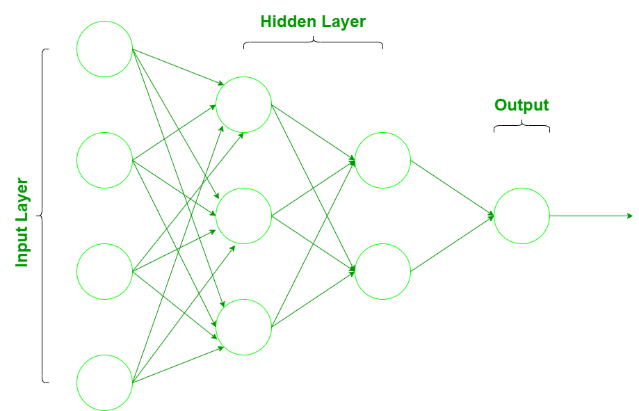
输入数据通过输入层被引入神经网络,输入层对于输入数据中存在的每个组件都有一个神经元,并与网络中存在的隐藏层(一个或多个)通信。之所以称为“隐藏”,是因为它们不构成输入或输出层。在隐藏层中,所有处理实际上都是通过一个以权重和偏差为特征的连接系统进行的(如前所述)。一旦接收到输入,神经元计算一个加权和,加上偏差,并根据结果和激活函数(最常见的是 sigmoid),它决定是否应该“触发”或“激活”。然后,神经元在称为“前向传递”的过程中将信息向下游传输到其他连接的神经元。在这个过程结束时,最后一个隐藏层连接到输出层,输出层对于每个可能的期望输出都有一个神经元。
在 R 编程中实现神经网络
使用 R 语言实现神经网络要容易得多,因为它里面有优秀的库。在用 R 实现神经网络之前,让我们先了解数据的结构。
了解数据的结构
在这里,让我们使用二进制数据集。目标是通过 gre、gpa 和排名等变量来预测候选人是否会被大学录取。 R 脚本是并排提供的,并带有注释以便更好地理解用户。数据为 .csv 格式。我们将使用getwd()函数获取工作目录,并在其中放置数据集 binary.csv 以继续进行。请在此处下载 csv 文件。
# preparing the dataset
getwd()
data <- read.csv("binary.csv" )
str(data)
输出:
'data.frame':   400 obs. of  4 variables:
 $ admit: int  0 1 1 1 0 1 1 0 1 0 ...
 $ gre  : int  380 660 800 640 520 760 560 400 540 700 ...
 $ gpa  : num  3.61 3.67 4 3.19 2.93 3 2.98 3.08 3.39 3.92 ...
 $ rank : int  3 3 1 4 4 2 1 2 3 2 ...
查看数据集的结构,我们可以观察到它有 4 个变量,其中,admit 告诉候选人是否会被录取(如果被录取,则为 1,如果未被录取,则为 0)gre、gpa 和 rank 给出候选人 gre 分数,他/她在以前的大学和以前的大学排名中的gpa。我们使用admit 作为因变量,使用gre、gpa 和rank 作为自变量。现在逐步了解整个过程
第 1 步:数据缩放
要为数据集建立神经网络,确保数据的适当缩放非常重要。数据的缩放是必不可少的,否则,一个变量可能仅仅因为它的规模而对预测变量产生很大的影响。使用未缩放的数据可能会导致毫无意义的结果。缩放数据的常用技术是 min-max 归一化、Z-score 归一化、中值和 MAD 以及 tan-h 估计器。最小-最大归一化将数据转换为一个公共范围,从而消除所有变量的缩放效应。在这里,我们使用 min-max 归一化来缩放数据。
# Draw a histogram for gre data
hist(data$gre)
输出: 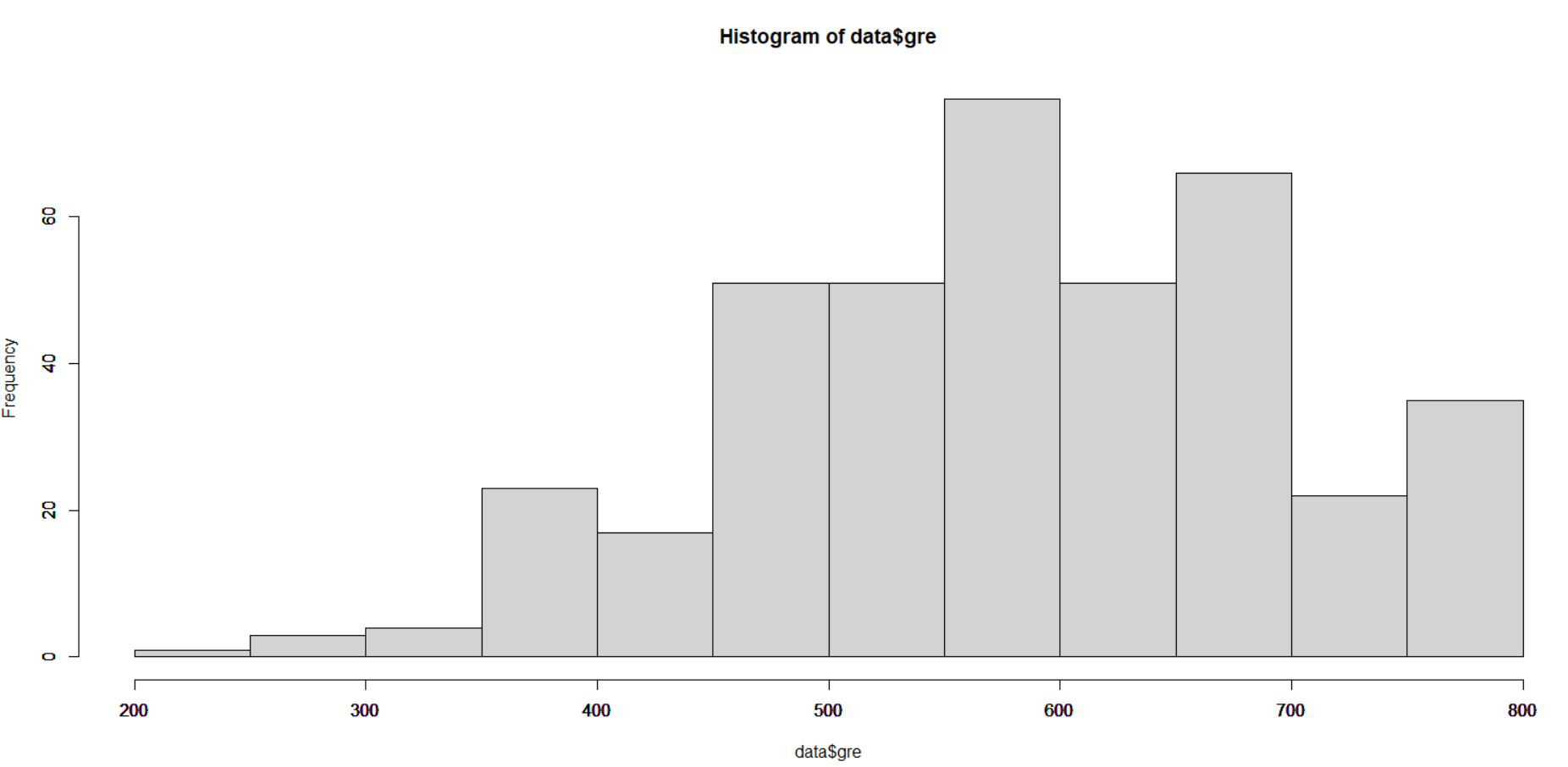
从上面 gre 的直方图我们可以看到 gre 从 200 到 800 不等。我们调用以下函数来规范化我们的数据:
normalize <- function(x) {
        return ((x - min(x)) / (max(x) - min(x)))
}
# Min-Max Normalization
data$gre <- (data$gre - min(data$gre)) / (max(data$gre) - min(data$gre))
hist(data$gre)
输出: 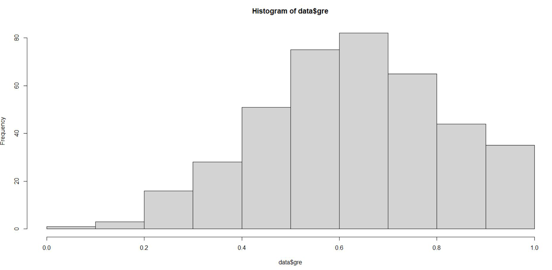
从上面的表示我们可以看到 gre 数据在 0 到 1 的范围内缩放。我们对 gpa 和 rank 做类似的事情。
# Min-Max Normalization
data$gpa <- (data$gpa - min(data$gpa)) / (max(data$gpa) - min(data$gpa))
hist(data$gpa)
data$rank <- (data$rank - min(data$rank)) / (max(data$rank) - min(data$rank))
hist(data$rank)
输出: 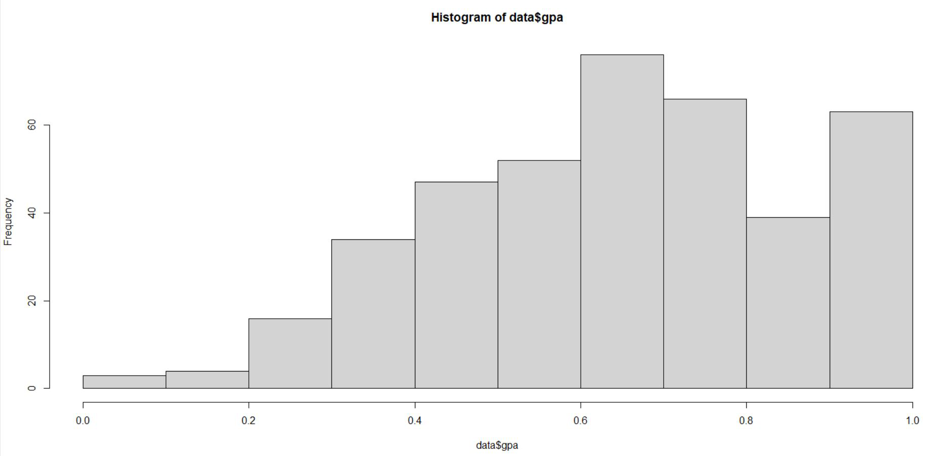
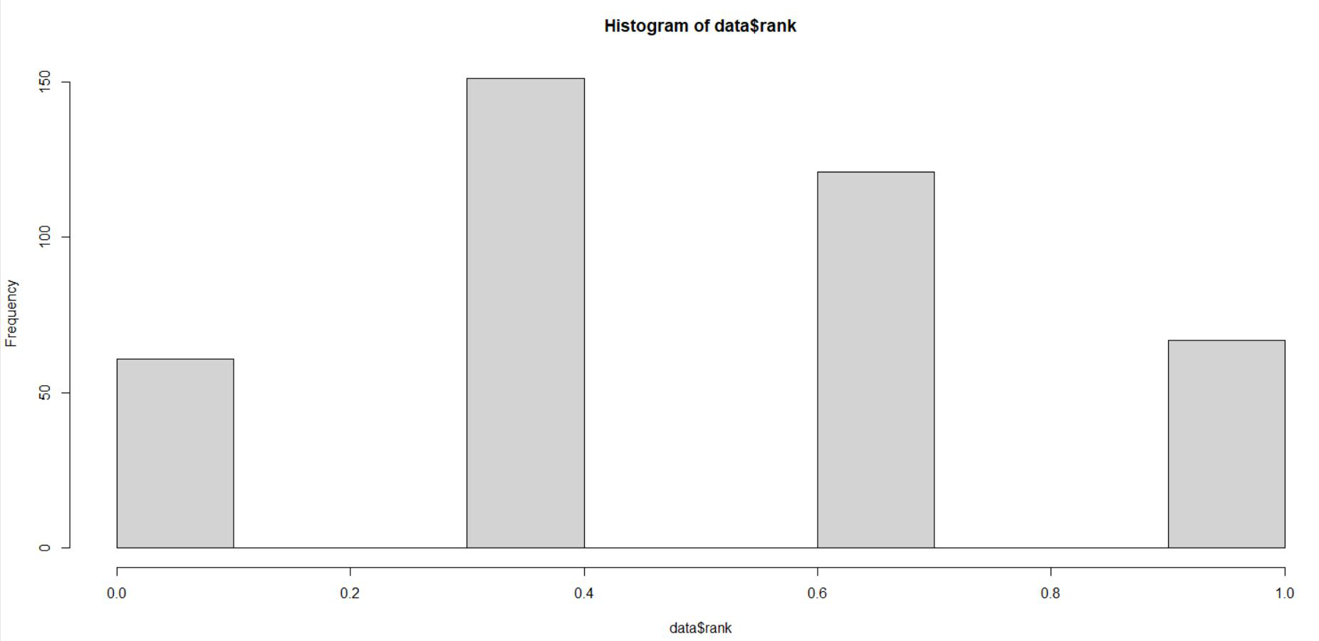
从以上两个直方图表示可以看出,gpa和rank也在0到1的范围内进行了缩放,缩放后的数据用于拟合神经网络。
第 2 步:数据采样
现在将数据分为训练集和测试集。训练集用于查找因变量和自变量之间的关系,而测试集用于分析模型的性能。我们使用 60% 的数据集作为训练集。使用随机抽样将数据分配给训练集和测试集。我们使用sample()函数对 R 执行随机抽样。每次使用set.seed()生成相同的随机样本并保持一致性。在拟合神经网络时使用索引变量来创建训练和测试数据集。 R脚本如下:
set.seed(222)
inp <- sample(2, nrow(data), replace = TRUE, prob = c(0.7, 0.3))
training_data <- data[inp==1, ]
test_data <- data[inp==2, ]
第 3 步:拟合神经网络
现在在我们的数据上拟合一个神经网络。我们同样使用神经网络库。 neuralnet()函数帮助我们为我们的数据建立一个神经网络。我们在这里使用的neuralnet()函数具有以下语法。
Syntax:
neuralnet(formula, data, hidden = 1, stepmax = 1e+05, rep = 1, lifesign = “none”, algorithm = “rprop+”, err.fct = “sse”, linear.output = TRUE)
参数:
| Argument | Description |
|---|---|
| formula | a symbolic description of the model to be fitted. |
| data | a data frame containing the variables specified in formula. |
| hidden | a vector of integers specifying the number of hidden neurons (vertices) in each layer |
| err.fct | a differentiable function that is used for the calculation of the error. Alternatively, the strings ‘sse’ and ‘ce’ which stand for the sum of squared errors and the cross-entropy can be used. |
| linear.output | logical. If act.fct should not be applied to the output neurons set linear output to TRUE, otherwise to FALSE. |
| lifesign | a string specifying how much the function will print during the calculation of the neural network. ‘none’, ‘minimal’ or ‘full’. |
| rep | the number of repetitions for the neural network’s training. |
| algorithm | a string containing the algorithm type to calculate the neural network. The following types are possible: ‘backprop’, ‘rprop+’, ‘rprop-‘, ‘sag’, or ‘slr’. ‘backprop’ refers to backpropagation, ‘rprop+’ and ‘rprop-‘ refer to the resilient backpropagation with and without weight backtracking, while ‘sag’ and ‘slr’ induce the usage of the modified globally convergent algorithm (grprop). |
| stepmax | the maximum steps for the training of the neural network. Reaching this maximum leads to a stop of the neural network’s training process. |
library(neuralnet)
set.seed(333)
n <- neuralnet(admit~gre + gpa + rank,
               data = training_data,
               hidden = 5,
               err.fct = "ce",
               linear.output = FALSE,
               lifesign = 'full',
               rep = 2,
               algorithm = "rprop+",
               stepmax = 100000)
hidden: 5    thresh: 0.01    rep: 1/2    steps:    1000 min thresh: 0.092244246452834
                                                   2000 min thresh: 0.092244246452834
                                                   3000 min thresh: 0.092244246452834
                                                   4000 min thresh: 0.092244246452834
                                                   5000 min thresh: 0.092244246452834
                                                   6000 min thresh: 0.092244246452834
                                                   7000 min thresh: 0.092244246452834
                                                   8000 min thresh: 0.0657773918077728
                                                   9000 min thresh: 0.0492128119805471
                                                  10000 min thresh: 0.0350341801886022
                                                  11000 min thresh: 0.0257113452845989
                                                  12000 min thresh: 0.0175961794629306
                                                  13000 min thresh: 0.0108791716102531
                                                  13253 error: 139.80883        time: 7.51 secs
hidden: 5    thresh: 0.01    rep: 2/2    steps:    1000 min thresh: 0.147257381292693
                                                   2000 min thresh: 0.147257381292693
                                                   3000 min thresh: 0.091389043508166
                                                   4000 min thresh: 0.0648814957085886
                                                   5000 min thresh: 0.0472858320232246
                                                   6000 min thresh: 0.0359632940146351
                                                   7000 min thresh: 0.0328699898176084
                                                   8000 min thresh: 0.0305035254157369
                                                   9000 min thresh: 0.0305035254157369
                                                  10000 min thresh: 0.0241743801258625
                                                  11000 min thresh: 0.0182557959333173
                                                  12000 min thresh: 0.0136844933371039
                                                  13000 min thresh: 0.0120885410813301
                                                  14000 min thresh: 0.0109156031403791
                                                  14601 error: 147.41304        time: 8.25 secs
从上面的输出我们得出结论,两个重复都收敛了。但是我们将在第一次重复中使用输出驱动,因为它给出的错误(139.80883)比第二次重复产生的错误(147.41304)少。现在,让我们绘制我们的神经网络并可视化计算的神经网络。
# plot our neural network
plot(n, rep = 1)
输出:
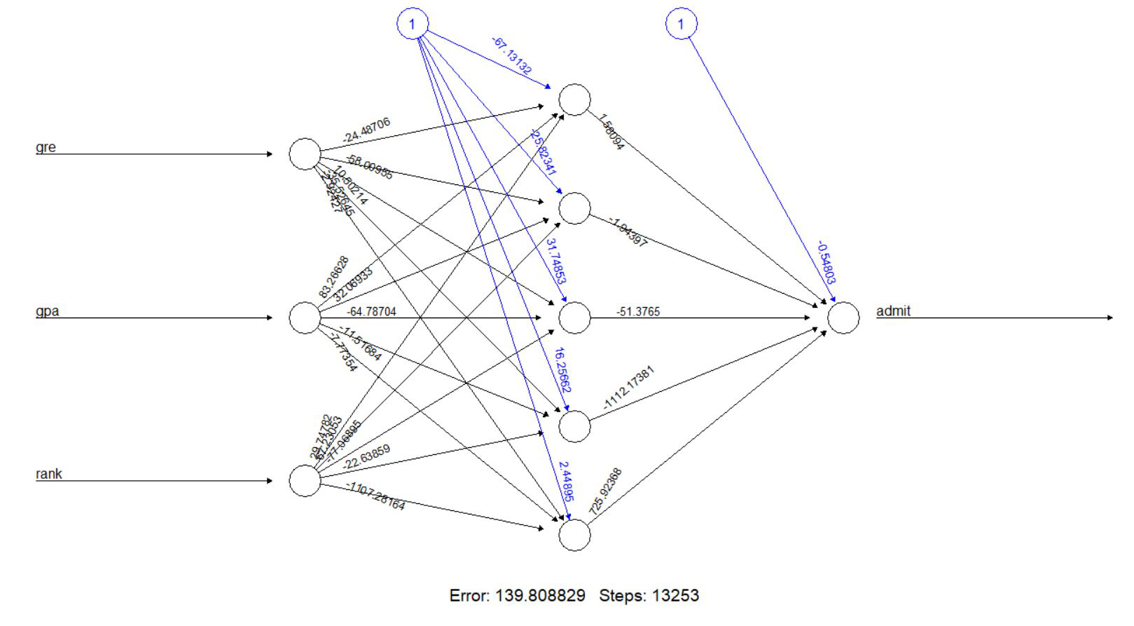
该模型在其隐藏层中有 5 个神经元。黑线显示与权重的连接。使用反向传播算法计算权重。蓝线显示偏差项(回归方程中的常数)。现在生成神经网络模型的误差,以及输入、隐藏层和输出之间的权重:
# error
n$result.matrix
输出:
[, 1]          [, 2]
error                  1.398088e+02  1.474130e+02
reached.threshold      9.143429e-03  9.970574e-03
steps                  1.325300e+04  1.460100e+04
Intercept.to.1layhid1 -6.713132e+01 -1.136151e+02
gre.to.1layhid1       -2.448706e+01  1.469138e+02
gpa.to.1layhid1        8.326628e+01  1.290251e+02
rank.to.1layhid1       2.974782e+01 -5.733805e+01
Intercept.to.1layhid2 -2.582341e+01  2.508958e-01
gre.to.1layhid2       -5.800955e+01  1.302115e+00
gpa.to.1layhid2        3.206933e+01 -4.856419e+00
rank.to.1layhid2       6.723053e+01  1.540390e+01
Intercept.to.1layhid3  3.174853e+01 -3.495968e+01
gre.to.1layhid3        1.050214e+01  1.325498e+02
gpa.to.1layhid3       -6.478704e+01 -4.536649e+01
rank.to.1layhid3      -7.706895e+01 -1.844943e+02
Intercept.to.1layhid4  1.625662e+01  2.188646e+01
gre.to.1layhid4       -3.552645e+01  1.956271e+01
gpa.to.1layhid4       -1.151684e+01  2.052294e+01
rank.to.1layhid4      -2.263859e+01  1.347474e+01
Intercept.to.1layhid5  2.448949e+00 -3.978068e+01
gre.to.1layhid5       -2.924269e+00 -1.569897e+02
gpa.to.1layhid5       -7.773543e+00  1.500767e+02
rank.to.1layhid5      -1.107282e+03  4.045248e+02
Intercept.to.admit    -5.480278e-01 -3.622384e+00
1layhid1.to.admit      1.580944e+00  1.717584e+00
1layhid2.to.admit     -1.943969e+00 -6.195182e+00
1layhid3.to.admit     -5.137650e+01  6.731498e+00
1layhid4.to.admit     -1.112174e+03 -4.245278e+00
1layhid5.to.admit      7.259237e+02  1.156083e+01
第 4 步:预测
让我们使用神经网络模型来预测评分。我们必须记住,预测评分将被缩放,并且必须对其进行转换,以便与实际评分进行比较。还将预测评分与实际评分进行比较。
# Prediction
output <- compute(n, rep = 1, training_data[, -1])
head(output$net.result)
输出:
[, 1]
2 0.34405929
3 0.41148373
4 0.07642387
7 0.98152454
8 0.26230256
9 0.07660906
head(training_data[1, ])
输出:
admit   gre      gpa      rank
2     1 0.7586207 0.8103448 0.6666667
第 5 步:混淆矩阵和误分类错误
然后,我们使用compute()方法对结果进行四舍五入,并创建一个混淆矩阵来比较真/假阳性和阴性的数量。我们将用训练数据形成一个混淆矩阵
# confusion Matrix $Misclassification error -Training data
output <- compute(n, rep = 1, training_data[, -1])
p1 <- output$net.result
pred1 <- ifelse(p1 > 0.5, 1, 0)
tab1 <- table(pred1, training_data$admit)
tab1
输出:
pred1 0   1
    0 177  58
    1  12  34
该模型生成 177 个真阴性(0)、34 个真阳性(1),同时有 12 个假阴性和 58 个假阳性。现在,让我们计算误分类误差(对于训练数据),其中 {1 – 分类误差}
1 - sum(diag(tab1)) / sum(tab1)
输出:
[1] 0.2491103
错误分类误差为 24.9%。我们可以通过增加隐藏层中的递减节点和偏差来进一步提高模型的准确性和效率。
机器学习算法的优势在于它们每次预测输出时都能学习和改进的能力。在神经网络的背景下,这意味着定义神经元之间连接的权重和偏差变得更加精确。这就是为什么选择权重和偏差的原因,例如网络的输出接近所有训练输入的真实值。同样,我们可以在 R 中制作更有效的神经网络模型来预测和推动决策。