使用 PyTorch 实现基于 CNN 的图像分类器

介绍：

由 Yann LeCun 在 1980 年代介绍的卷积神经网络（也称为 CNN 或 ConvNet）已经走过了漫长的道路。从被用于简单的数字分类任务开始，基于 CNN 的架构正被广泛用于许多深度学习和计算机视觉相关的任务，如对象检测、图像分割、注视跟踪等。使用 PyTorch 框架，本文将在流行的 CIFAR-10 数据集上实现基于 CNN 的图像分类器。

在继续代码和安装之前，希望读者了解 CNN 在理论上是如何工作的，以及卷积、池化等各种相关操作。本文还假设您基本熟悉 PyTorch 工作流程及其各种实用程序，例如 Dataloaders，数据集、张量转换和 CUDA 操作。为了快速复习这些概念，我们鼓励读者阅读以下文章：

• 卷积神经网络简介
• 使用 PyTorch 通过验证训练神经网络
• 如何在 Pytorch 中设置和运行 CUDA 操作？

安装

为了实现 CNN 和下载 CIFAR-10 数据集，我们将需要torch和torchvision模块。除此之外，我们将使用 numpy 和 matplotlib 进行数据分析和绘图。可以使用 pip 包管理器通过以下命令安装所需的库：

    pip install torch torchvision torchaudio numpy matplotlib

逐步实施

第 1 步：从训练集中下载数据并打印一些样本图像。

• 在开始实施 CNN 之前，我们首先需要将数据集下载到我们的本地机器上，我们将在上面训练我们的模型。为此，我们将使用torchvision实用程序，并将 CIFAR-10 数据集下载到目录“./CIFAR10/train”和“./CIFAR10/test ”中的训练和测试集中。我们还应用了归一化变换，其中该过程在所有图像的三个通道上完成。
• 现在，我们有一个训练数据集和一个测试数据集，分别包含 50000 和 10000 张图像，尺寸为 32x32x3。之后，我们将这些数据集转换为批量大小为 128 的数据加载器，以实现更好的泛化和更快的训练过程。
• 最后，我们从第一个训练批次中绘制出一些样本图像，以了解我们使用torchvision的make_grid实用程序处理的图像。

代码：

Python3

import torch
import torchvision
import matplotlib.pyplot as plt
import numpy as np
  
# The below two lines are optional and are just there to avoid any SSL
# related errors while downloading the CIFAR-10 dataset
import ssl
ssl._create_default_https_context = ssl._create_unverified_context
  
#Defining plotting settings
plt.rcParams['figure.figsize'] = 14, 6
  
#Initializing normalizing transform for the dataset
normalize_transform = torchvision.transforms.Compose([
    torchvision.transforms.ToTensor(),
    torchvision.transforms.Normalize(mean = (0.5, 0.5, 0.5), 
                                     std = (0.5, 0.5, 0.5))])
  
#Downloading the CIFAR10 dataset into train and test sets
train_dataset = torchvision.datasets.CIFAR10(
    root="./CIFAR10/train", train=True,
    transform=normalize_transform,
    download=True)
    
test_dataset = torchvision.datasets.CIFAR10(
    root="./CIFAR10/test", train=False,
    transform=normalize_transform,
    download=True)
    
#Generating data loaders from the corresponding datasets
batch_size = 128
train_loader = torch.utils.data.DataLoader(train_dataset, batch_size=batch_size)
test_loader = torch.utils.data.DataLoader(test_dataset, batch_size=batch_size)
  
#Plotting 25 images from the 1st batch 
dataiter = iter(train_loader)
images, labels = dataiter.next()
plt.imshow(np.transpose(torchvision.utils.make_grid(
  images[:25], normalize=True, padding=1, nrow=5).numpy(), (1, 2, 0)))
plt.axis('off')

输出：

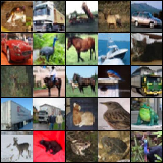
图 1：来自训练数据集的一些示例图像

步骤 2：绘制数据集的类分布

绘制出训练集的类分布通常是一个好主意。这有助于检查提供的数据集是否平衡。为此，我们分批迭代整个训练集并收集每个实例的相应类。最后，我们计算唯一类的数量并绘制它们。

代码：

Python3

#Iterating over the training dataset and storing the target class for each sample
classes = []
for batch_idx, data in enumerate(train_loader, 0):
    x, y = data 
    classes.extend(y.tolist())
      
#Calculating the unique classes and the respective counts and plotting them
unique, counts = np.unique(classes, return_counts=True)
names = list(test_dataset.class_to_idx.keys())
plt.bar(names, counts)
plt.xlabel("Target Classes")
plt.ylabel("Number of training instances")

输出：

图 2：训练集的类分布

如图 2 所示，十个类中的每一类都有几乎相同数量的训练样本。因此，我们不需要采取额外的步骤来重新平衡数据集。

第 3 步：实现 CNN 架构

在架构方面，我们将使用一个简单的模型，该模型使用三个深度分别为32、64 和 64 的卷积层，然后是两个完全连接的层来执行分类。

• 每个卷积层都涉及一个涉及3×3 卷积滤波器的卷积操作，然后是一个 ReLU 激活操作，用于将非线性引入系统，以及一个带有 2×2 滤波器的最大池操作，以降低特征图的维数。
• 在卷积块结束后，我们将多维层展平为低维结构，用于开始我们的分类块。在第一个线性层之后，最后一个输出层（也是一个线性层）对于我们数据集中的十个唯一类中的每一个都有十个神经元。

架构如下：

图 3：CNN 的架构

为了构建我们的模型，我们将创建一个继承自torch.nn.Module类的CNN 类，以利用 Pytorch 实用程序。除此之外，我们将使用torch.nn.Sequential容器一个接一个地组合我们的层。

• Conv2D()、ReLU()和MaxPool2D()层执行卷积、激活和池化操作。我们使用 1 的填充为内核提供足够的学习空间，因为填充为图像提供了更多的覆盖区域，尤其是外帧中的像素。
• 在卷积块之后， Linear()全连接层执行分类。

代码：

Python3

class CNN(torch.nn.Module):
    def __init__(self):
        super().__init__()
        self.model = torch.nn.Sequential(
            #Input = 3 x 32 x 32, Output = 32 x 32 x 32
            torch.nn.Conv2d(in_channels = 3, out_channels = 32, kernel_size = 3, padding = 1), 
            torch.nn.ReLU(),
            #Input = 32 x 32 x 32, Output = 32 x 16 x 16
            torch.nn.MaxPool2d(kernel_size=2),
  
            #Input = 32 x 16 x 16, Output = 64 x 16 x 16
            torch.nn.Conv2d(in_channels = 32, out_channels = 64, kernel_size = 3, padding = 1),
            torch.nn.ReLU(),
            #Input = 64 x 16 x 16, Output = 64 x 8 x 8
            torch.nn.MaxPool2d(kernel_size=2),
              
            #Input = 64 x 8 x 8, Output = 64 x 8 x 8
            torch.nn.Conv2d(in_channels = 64, out_channels = 64, kernel_size = 3, padding = 1),
            torch.nn.ReLU(),
            #Input = 64 x 8 x 8, Output = 64 x 4 x 4
            torch.nn.MaxPool2d(kernel_size=2),
  
            torch.nn.Flatten(),
            torch.nn.Linear(64*4*4, 512),
            torch.nn.ReLU(),
            torch.nn.Linear(512, 10)
        )
  
    def forward(self, x):
        return self.model(x)

第 4 步：定义训练参数并开始训练过程

我们通过选择将模型训练到的设备（即 CPU 或 GPU）来开始训练过程。然后，我们定义我们的模型超参数，如下所示：

• 我们训练我们的模型超过50 个时期，并且由于我们有一个多类问题，我们使用交叉熵损失作为我们的目标函数。
• 我们使用流行的Adam 优化器，学习率为 0.001 ， weight_decay 为 0.01 ，通过正则化来优化目标函数来防止过度拟合。

最后，我们开始我们的训练循环，包括通过比较预测标签和真实标签来计算每个批次的输出和损失。最后，我们绘制了每个时期的训练损失，以确保训练过程按计划进行。

代码：

Python3

#Selecting the appropriate training device
device = 'cuda' if torch.cuda.is_available() else 'cpu'
model = CNN().to(device)
  
#Defining the model hyper parameters
num_epochs = 50
learning_rate = 0.001
weight_decay = 0.01
criterion = torch.nn.CrossEntropyLoss()
optimizer = torch.optim.Adam(model.parameters(), lr=learning_rate, weight_decay=weight_decay)
  
#Training process begins
train_loss_list = []
for epoch in range(num_epochs):
    print(f'Epoch {epoch+1}/{num_epochs}:', end = ' ')
    train_loss = 0
      
    #Iterating over the training dataset in batches
    model.train()
    for i, (images, labels) in enumerate(train_loader):
          
        #Extracting images and target labels for the batch being iterated
        images = images.to(device)
        labels = labels.to(device)
  
        #Calculating the model output and the cross entropy loss
        outputs = model(images)
        loss = criterion(outputs, labels)
  
        #Updating weights according to calculated loss
        optimizer.zero_grad()
        loss.backward()
        optimizer.step()
        train_loss += loss.item()
      
    #Printing loss for each epoch
    train_loss_list.append(train_loss/len(train_loader))
    print(f"Training loss = {train_loss_list[-1]}")   
      
#Plotting loss for all epochs
plt.plot(range(1,num_epochs+1), train_loss_list)
plt.xlabel("Number of epochs")
plt.ylabel("Training loss")

输出：

图 4：训练损失与 epoch 数的关系图

从图 4 中，我们可以看到损失随着 epoch 的增加而减少，这表明训练过程是成功的。

Step-5：计算模型在测试集上的准确度

现在我们的模型已经训练好了，我们需要检查它在测试集上的表现。为此，我们分批迭代整个测试集，并通过比较每个批次的真实标签和预测标签来计算准确度得分。

代码：

Python3

test_acc=0
model.eval()
  
with torch.no_grad():
    #Iterating over the training dataset in batches
    for i, (images, labels) in enumerate(test_loader):
          
        images = images.to(device)
        y_true = labels.to(device)
          
        #Calculating outputs for the batch being iterated
        outputs = model(images)
          
        #Calculated prediction labels from models
        _, y_pred = torch.max(outputs.data, 1)
          
        #Comparing predicted and true labels
        test_acc += (y_pred == y_true).sum().item()
      
    print(f"Test set accuracy = {100 * test_acc / len(test_dataset)} %")

输出：

图 5：测试集的准确度

第 6 步：为测试集中的样本图像生成预测

如图 5 所示，我们的模型达到了近 72% 的准确率。为了验证它的性能，我们可以为一些样本图像生成一些预测。为此，我们获取最后一批测试集的前五张图像，并使用 torchvision 的make_grid实用程序绘制它们。然后，我们从模型中收集他们的真实标签和预测，并在情节标题中显示它们。

代码：

Python3

#Generating predictions for 'num_images' amount of images from the last batch of test set
num_images = 5
y_true_name = [names[y_true[idx]] for idx in range(num_images)] 
y_pred_name = [names[y_pred[idx]] for idx in range(num_images)] 
  
#Generating the title for the plot
title = f"Actual labels: {y_true_name}, Predicted labels: {y_pred_name}"
  
#Finally plotting the images with their actual and predicted labels in the title
plt.imshow(np.transpose(torchvision.utils.make_grid(images[:num_images].cpu(), normalize=True, padding=1).numpy(), (1, 2, 0)))
plt.title(title)
plt.axis("off")

输出：

图 6：来自测试集的 5 个样本图像的实际标签与预测标签。请注意，标签的顺序与相应图像的顺序相同，从左到右。

从图 6 中可以看出，该模型对除了第二张图像之外的所有图像都产生了正确的预测，因为它将狗错误地分类为猫！

结论：

本文介绍了在流行的 CIFAR-10 数据集上简单 CNN 的 PyTorch 实现。鼓励读者尝试使用网络架构和模型超参数，以进一步提高模型的准确性！

参考

1. https://cs231n.github.io/convolutional-networks/
2. https://pytorch.org/docs/stable/index.html
3. https://pytorch.org/tutorials/beginner/blitz/cifar10_tutorial.html