Seaborn 中的多图网格

先决条件： Matplotlib、Seaborn

在本文中，我们将看到多维绘图数据，这是一种在数据集的不同子集上绘制同一绘图的多个实例的有用方法。它允许查看者快速提取有关复杂数据集的大量信息。在 Seaborn 中，我们将通过两种方式在单个窗口中绘制多个图形。首先借助 Facetgrid()函数和其他隐式借助 matplotlib。

FacetGrid： FacetGrid 是一种基于函数绘制网格的通用方法。它有助于可视化一个变量的分布以及多个变量之间的关系。它的对象使用数据框作为输入和塑造网格的列、行或颜色维度的变量的名称，语法如下：

Syntax: seaborn.FacetGrid( data, \*\*kwargs)

• data: Tidy dataframe where each column is a variable and each row is an observation.
• \*\*kwargs: It uses many arguments as input such as, i.e. row, col, hue, palette etc.

下面是上述方法的实现：

导入所有需要的Python库

Python3

import seaborn as sns
import numpy as np
import pandas as pd
import matplotlib.pyplot as plt

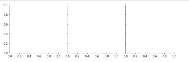
示例 1：在这里，我们像这样初始化网格以设置 matplotlib 图形和轴，但没有在它们上绘制任何东西，我们使用的是习题数据集，它是众所周知的数据集，可用作 seaborn 中的内置数据集。
该类的基本用法与 FacetGrid 非常相似。首先初始化网格，然后将绘图函数传递给 map 方法，它将在每个子图上调用。

蟒蛇3

# loading of a dataframe from seaborn
exercise = sns.load_dataset("exercise")
  
# Form a facetgrid using columns
sea = sns.FacetGrid(exercise, col = "time")

输出：

示例 2：此函数将绘制图形并注释轴。要制作关系图，首先初始化网格，然后将绘图函数传递给 map 方法，它将在每个子图上调用。

蟒蛇3

# Form a facetgrid using columns with a hue 
sea = sns.FacetGrid(exercise, col = "time", hue = "kind")
    
# map the above form facetgrid with some attributes   
sea.map(sns.scatterplot, "pulse", "time", alpha = .8)
  
# adding legend
sea.add_legend()

输出：

示例 3：有几个选项可用于控制可以传递给类构造函数的网格外观。

蟒蛇3

sea = sns.FacetGrid(exercise, row = "diet",
                    col = "time", margin_titles = True)
  
sea.map(sns.regplot, "id", "pulse", color = ".3",
        fit_reg = False, x_jitter = .1)

输出：

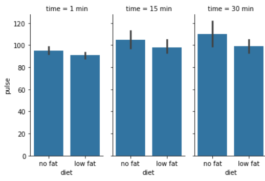
示例 4：通过提供每个面的高度以及纵横比来设置图形的大小：

蟒蛇3

sea = sns.FacetGrid(exercise, col = "time",
                    height = 4, aspect  =.5)
  
sea.map(sns.barplot, "diet", "pulse",
        order = ["no fat", "low fat"])

输出：

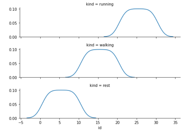
示例 5： facet 的默认排序源自 DataFrame 中的信息。如果用于定义分面的变量具有分类类型，则使用分类的顺序。否则，构面将按照类别级别的出现顺序排列。但是，可以使用适当的 *_order 参数指定任何方面维度的排序：

蟒蛇3

exercise_kind = exercise.kind.value_counts().index
sea = sns.FacetGrid(exercise, row = "kind", 
                    row_order = exercise_kind,
                    height = 1.7, aspect = 4)
  
sea.map(sns.kdeplot, "id")

输出：

示例 6：如果您有多个级别的一个变量，您可以沿列绘制它，但“包装”它们，使它们跨越多行。这样做时，您不能使用行变量。

蟒蛇3

g = sns.PairGrid(exercise)
g.map_diag(sns.histplot)
g.map_offdiag(sns.scatterplot)

输出：

示例 7：

在这个例子中，我们将看到我们还可以在 pairplot()函数的帮助下绘制多图网格。这将 DataFrame 中变量的 (n, 2) 组合的关系显示为图矩阵，对角线图是单变量图。

蟒蛇3

# importing packages 
import seaborn 
import matplotlib.pyplot as plt 
  
# loading dataset using seaborn 
df = seaborn.load_dataset('tips') 
  
# pairplot with hue sex 
seaborn.pairplot(df, hue ='size') 
plt.show() 

输出

方法二：隐式借助matplotlib。

在本文中，我们将学习如何使用matplotlib 和 seabor n 创建子图。

导入所有需要的Python库

蟒蛇3

import seaborn as sns
import numpy as np
import pandas as pd
import matplotlib.pyplot as plt
  
# Setting seaborn as default style even
# if use only matplotlib
sns.set()

示例 1：在这里，我们在不带参数的情况下初始化网格返回一个图形和一个轴，我们可以使用下面的语法对其进行解包。

蟒蛇3

figure, axes = plt.subplots()
figure.suptitle('Geeksforgeeks - one axes with no data')

输出：

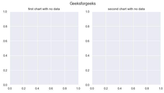
示例 2：在此示例中，我们创建了一个 1 行 2 列的图，仍然没有传递数据，即 nrows 和 ncols。如果按此顺序给出，我们不需要键入 arg 名称，只需键入其值。

• figsize设置我们图形的总尺寸。
• sharex和sharey用于在图表之间共享一个或两个轴。

蟒蛇3

figure, axes = plt.subplots(1, 2, sharex=True, figsize=(10,5))
figure.suptitle('Geeksforgeeks')
axes[0].set_title('first chart with no data')
axes[1].set_title('second chart with no data')

输出：

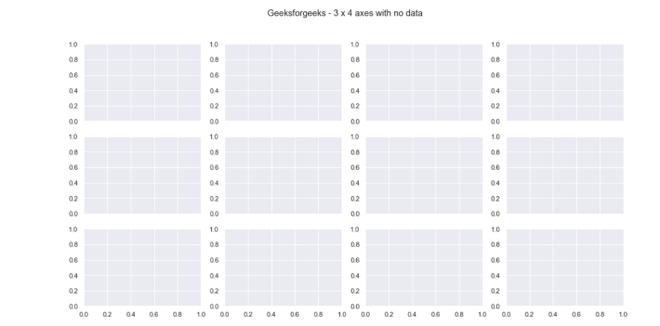
示例 3：如果您有多个级别

蟒蛇3

figure, axes = plt.subplots(3, 4, sharex=True, figsize=(16,8))
figure.suptitle('Geeksforgeeks - 3 x 4 axes with no data')

输出

示例 4：在这里，我们正在初始化 matplotlib 图形和坐标轴，在此示例中，我们在运动数据集的帮助下传递所需的数据，该数据集是一个众所周知的数据集，可用作 seaborn 中的内置数据集。通过使用此方法，您可以借助 seaborn 中的 matplotlib，通过隐式行和列绘制任意数量的多图网格和任何样式的图形。我们在这里使用 sns.boxplot，我们需要使用轴变量中的对应元素设置参数。

蟒蛇3

import seaborn as sns
import numpy as np
import pandas as pd
import matplotlib.pyplot as plt
  
  
fig, axes = plt.subplots(2, 3, figsize=(18, 10))
  
fig.suptitle('Geeksforgeeks - 2 x 3 axes Box plot with data')
  
iris = sns.load_dataset("iris")
  
sns.boxplot(ax=axes[0, 0], data=iris, x='species', y='petal_width')
sns.boxplot(ax=axes[0, 1], data=iris, x='species', y='petal_length')
sns.boxplot(ax=axes[0, 2], data=iris, x='species', y='sepal_width')
sns.boxplot(ax=axes[1, 0], data=iris, x='species', y='sepal_length')
sns.boxplot(ax=axes[1, 1], data=iris, x='species', y='petal_width')
sns.boxplot(ax=axes[1, 2], data=iris, x='species', y='petal_length')

输出：

示例 5： gridspec() 用于具有某些指定宽度和高度空间的行和列网格。 plt.GridSpec 对象本身不会创建绘图，但它只是一个方便的接口，可被 subplot() 命令识别。

蟒蛇3

import matplotlib.pyplot as plt
  
Grid_plot = plt.GridSpec(2, 3, wspace = 0.8,
                         hspace = 0.6)
  
plt.subplot(Grid_plot[0, 0])
plt.subplot(Grid_plot[0, 1:])
plt.subplot(Grid_plot[1, :2])
plt.subplot(Grid_plot[1, 2])

输出：

示例 6：这里我们将使用 subplots() 创建一个 3×4 的子图网格，其中同一行中的所有轴共享其 y 轴比例，同一列中的所有轴共享其 x 轴比例。

蟒蛇3

import matplotlib.pyplot as plt
  
figure, axes = plt.subplots(3, 4,
                            figsize = (15, 10))
  
figure.suptitle('Geeksforgeeks - 2 x 3 axes grid plot using subplots')

输出：