- R随机森林(1)
- R-随机森林
- 随机森林python(1)
- 随机森林python代码示例
- R 编程中的随机森林方法
- R 编程中的随机森林方法(1)
- Python中的随机森林回归(1)
- 随机森林回归器 python (1)
- Python中的随机森林回归
- 随机森林回归器 python 代码示例
- 如何构建随机森林 - R 编程语言(1)
- sklearn 随机森林 - Python 代码示例
- python中的随机森林分类器(1)
- 分类算法-随机森林
- 分类算法-随机森林(1)
- 如何构建随机森林 - R 编程语言代码示例
- stackoverflow python 随机森林 - Python (1)
- python代码示例中的随机森林分类器
- stackoverflow python 随机森林 - Python 代码示例
- R 编程中回归的随机森林方法(1)
- R 编程中回归的随机森林方法
- 随机森林分类器的超参数(1)
- 随机森林分类器的超参数
- scikit 学习随机森林 - Python (1)
- 机器学习-随机森林算法
- 机器学习-随机森林算法(1)
- 如何在 R 中创建森林图?
- 如何在 R 中创建森林图?(1)
- scikit 学习随机森林 - Python 代码示例
📅 最后修改于: 2021-01-08 10:10:33 🧑 作者: Mango
R-随机森林
随机森林也称为决策树森林。它是流行的基于决策树的集成模型之一。这些模型的准确性高于其他决策树。该算法可用于分类和回归应用。
在一个随机森林中,我们创建了大量决策树,并且在每个决策树中,每个观察结果都得到反馈。最终输出是每个观察结果最常见的结果。通过向所有树木提供新的观察结果,我们为每种分类模型投了多数票。
对于在构造树时未使用的情况进行了错误估计。这被称为袋外(OOB)错误估计,以百分比表示。
决策树易于过度拟合,这是它的主要缺点。原因是,如果加深了树木,它们就能适应数据中所有类型的变化,包括噪声。可以通过部分修剪来解决此问题,并且结果通常不尽人意。
R允许我们通过提供randomForest包来创建随机森林。 randomForest软件包提供了randomForest()函数,可帮助我们创建和分析随机森林。 R中的随机森林有以下语法:
randomForest(formula, data)
例:
让我们开始了解如何使用randomForest包及其函数。为此,我们举一个使用心脏疾病数据集的示例。让我们逐步开始编码部分。
1)第一步,我们必须加载三个必需的库,即ggplot2,cowplot和randomForest。
#Loading ggplot2, cowplot, and randomForest packages
library(ggplot2)
library(cowplot)
library(randomForest)
2)现在,我们将使用http://archive.ics.uci.edu/ml/machine-learning-databases/heart-disease/processed.cleveland.data中存在的心脏病数据集。然后,我们从该数据集中读取CSV格式的数据,并将其存储在变量中。
#Fetching heart-disease dataset
url<-"http://archive.ics.uci.edu/ml/machine-learning-databases/heart-disease/processed.cleveland.data"
data <- read.csv(url,header=FALSE)
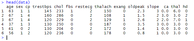
3)现在,我们在head()函数的帮助下print数据,该函数仅将开始的六行打印为:
#Head print six rows of data.
head(data)
当我们运行上面的代码时,它将生成以下输出。
输出:

4)从上面的输出中,很明显没有任何列被标记。现在,我们命名这些列,并使用以下方式标记这些列:
colnames(data) <-c("age","sex","cp","trestbps","chol","fbs","restecg","thalach","exang","oldpeak","slope","ca","thal","hd")
head(data)
输出:
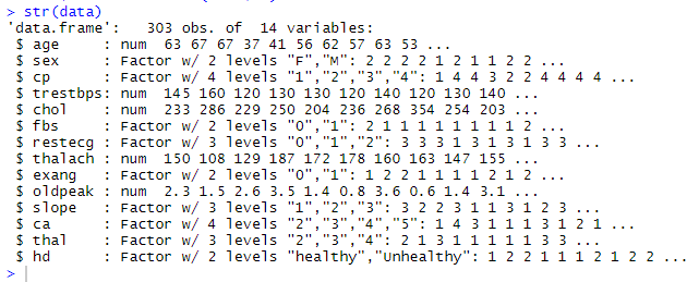
5)让我们借助str()函数检查数据结构以更好地分析数据。
str(data)
输出:

6)在上面的输出中,我们突出显示将在分析中使用的那些列。从输出中很明显,有些列被弄乱了。性别被认为是一个因素,其中0代表“女性”,而1代表“男性”。 cp(胸部疼痛)也被认为是一个因素,其中1到3级代表不同类型的疼痛,而4级代表无胸痛。
ca和thal是因素,但水平之一是“?”当我们需要它成为不适用时。我们必须清理数据集中的数据,如下所示:
#Changing the "?" to NAs?
data[data=="?"] <- NA

#Converting the 0's in sex to F and 1's to M
data[data$sex==0,]$sex <-"F"
data[data$sex==1,]$sex <-"M"

#Converting columns tnto the factors
data$sex<- as.factor(data$sex)
data$cp<- as.factor(data$cp)
data$fbs<- as.factor(data$fbs)
data$restecg<- as.factor(data$restecg)
data$exang<- as.factor(data$exang)
data$slope<- as.factor(data$slope)

#ca and thal columns contain? rather than NA. R treats it as a column of string, We correct this assumption by telling R that is a column of integers.

data$ca<- as.integer(data$ca)
data$ca<- as.factor(data$ca)
data$thal<- as.integer(data$thal)
data$thal<- as.factor(data$thal)

#Making data hd where 0's represent healthy and 1's to unhealthy.
data$hd<- ifelse(test=data$hd==0,yes="healthy",no="Unhealthy")
data$hd<- as.factor(data$hd)

#Checking structure of data
str(data)
输出:
7)现在,我们通过设置随机数生成器的种子来随机采样事物,以便我们可以再现结果。
set.seed(42)
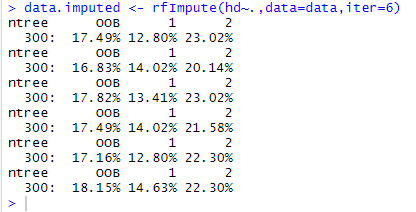
8)NWxt,我们使用rfImput()函数为数据集中的NA赋值。通过以下方式:
data.imputed<- rfImpute(hd~.,data=data,iter=6)
输出:
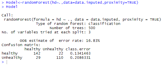
9)现在,我们以下列方式借助randomForest()函数构建适当的随机森林:
Model<-randomForest(hd~.,data=data.imputed,ntree=1000,proximity=TRUE)
Model
输出:
10)现在,如果500棵树足以进行最佳分类,我们将绘制错误率。我们创建一个数据帧,它将以以下方式格式化错误率信息:
oob_error_data<- data.frame(Trees=rep(1:nrow(Model$err.rate),times=3),Type=rep(c("OOB","Healthy","Unhealthy"),each=nrow(Model$err.rate)),Error=c(Model$err.rate[,"OOB"],Model$err.rate[,"healthy"],Model$err.rate[,"Unhealthy"]))
11)我们通过以下方式调用ggplot绘制错误率:
11)     We call the ggplot for plotting error rate in the following way:
ggplot(data=oob_error_data,aes(x=Trees,y=Error))+geom_line(aes(color=Type))
输出:
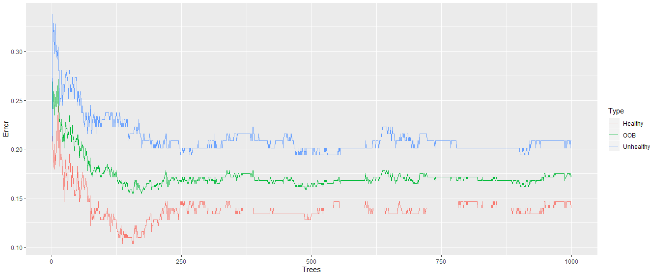
从上面的输出中可以明显看出,当我们的随机森林中有更多的树时,错误率会降低。
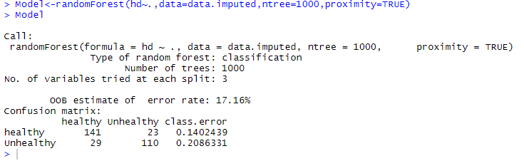
12)现在,我们添加1000棵树,并检查错误率会进一步下降吗?因此,我们创建了一个包含1000棵树的随机森林,并像以前一样找到了错误率。
Model<-randomForest(hd~.,data=data.imputed,ntree=1000,proximity=TRUE)
Model
输出:
oob_error_data<- data.frame(Trees=rep(1:nrow(Model$err.rate),times=3),Type=rep(c("OOB","Healthy","Unhealthy"),each=nrow(Model$err.rate)),Error=c(Model$err.rate[,"OOB"],Model$err.rate[,"healthy"],Model$err.rate[,"Unhealthy"]))
ggplot(data=oob_error_data,aes(x=Trees,y=Error))+geom_line(aes(color=Type))
输出:

从上面的输出可以明显看出,错误率已稳定下来。
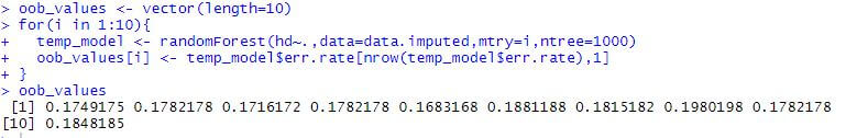
13)现在,我们需要确保我们正在考虑树中每个内部节点的最佳变量数。这将通过以下方式完成:
#Creating a vector that can hold ten values.
oob_values<- vector(length=10)

#Testing of the different numbers of variables at each step.
for(i in 1:10){
  #Building a random forest for determining the number of variables to try at each step.
temp_model<- randomForest(hd~.,data=data.imputed,mtry=i,ntree=1000)

  #Storing OOB error rate.
oob_values[i] <- temp_model$err.rate[nrow(temp_model$err.rate),1]
}
oob_values
输出:
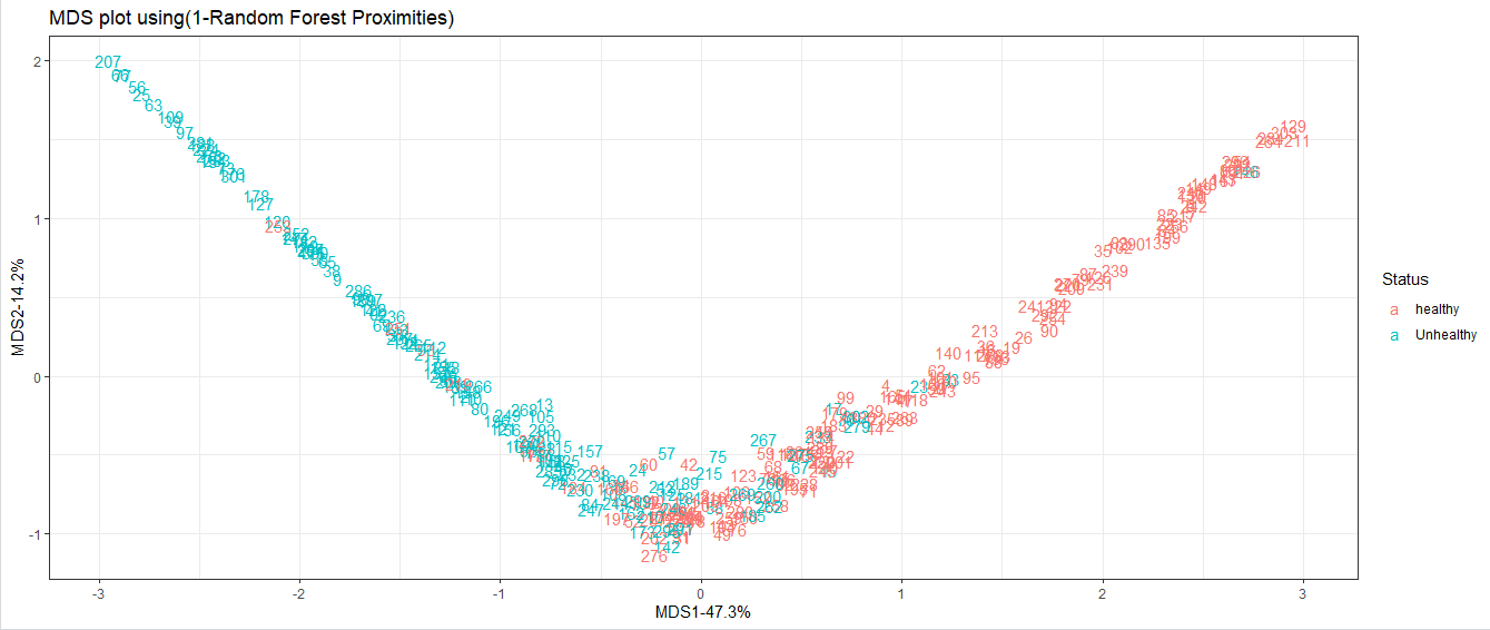
14)现在,我们使用随机森林绘制带有样本的MDS图。这将向我们展示它们之间的相互关系。这将通过以下方式完成:
#Creating a distance matrix with the help of dist() function.
distance_matrix<- dist(1-Model$proximity)

#Running cmdscale() on the distance matrix.
mds_stuff<- cmdscale(distance_matrix,eig=TRUE,x.ret=TRUE)

#Calculating the percentage of variation in the distance matrix that the X and Y axes account for.
mds_var_per<- round(mds_stuff$eig/sum(mds_stuff$eig)*100,1)

#Formatting the data for ggplot() function
mds_values<- mds_stuff$points
mds_data<- data.frame(Sample=rownames(mds_values),X=mds_values[,1],Y=mds_values[,2],Status=data.imputed$hd)

#Drawing the graph with ggplot() function.
ggplot(data=mds_data,aes(x=X,y=Y,label=Sample))+geom_text(aes(color=Status))+theme_bw()+xlab(paste("MDS1-",mds_var_per[1],"%",sep=""))+ylab(paste("MDS2-",mds_var_per[2],"%",sep=""))+ggtitle("MDS plot using(1-Random Forest Proximities)")
输出: