使用Turicreate了解高杠杆点

高杠杆点：如果数据点具有极高的预测值输入值，则将其视为高杠杆点。与整个数据集中的其他数据点相比，极限输入值仅意味着极低或极高的值。之所以在机器学习中引入这样的概念，是因为它可能会极大地影响模型对特定数据的拟合。

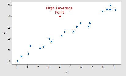
高杠杆点的例子

In this tutorial we are going to use turicreate to understand the concept of a high leverage point, so make sure you have turicreate installed in your system in order to follow along with the tutorial. For more info on Turicreate you can check this nice article on Turicreate.

因此，让我们逐步了解这个概念。

步骤1：我们将从导入本教程中需要的所有必需库开始。

• Turicreate用于拟合我们的回归模型。
• Matplotlib用于可视化数据。
• 随机产生的随机数。

Python3

import turicreate 
import matplotlib.pyplot as plt
import random

步骤2：接下来，我们将生成一些数据以适合我们的模型，并使用matplotlib可视化数据。

Python3

#Creating data point for this tutorial
X = [random.randrange(1, 150) for i in range(200)]
Y = [random.randrange(200, 3000) for i in range(200)]
  
#Creating a separate point to demonstrate high leverage points
X.append(400)
Y.append(1000)
  
#Creating a SArray and SFRame
Xs = turicreate.SArray(X)
Ys = turicreate.SArray(Y)
data_points = turicreate.SFrame({"X" : Xs, "Y" : Ys})
  
#Plotting the Data
plt.scatter(Xs, Ys)
plt.xlabel("Input")
plt.ylabel("Output")
plt.show()

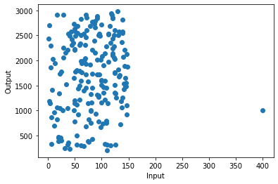
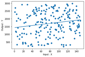
输出

正如您在图像中看到的那样，与其他数据相比，在(400,1000)坐标中有一个沿x轴非常远的点。该点称为高杠杆点。

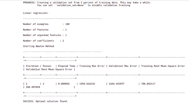
步骤3：现在，我们将在数据上拟合回归模型。

Python3

#Fitting a linear Regression model with the given data
model = turicreate.linear_regression.create(data_points, 
                                            target = "Y", 
                                            features = ["X"])
  
#Plotting the fitted model
plt.scatter(data_points["X"], data_points["Y"])
plt.xlabel("Input : X")
plt.ylabel("Output : Y")
plt.plot(data_points["X"], model.predict(data_points))
plt.show()

输出

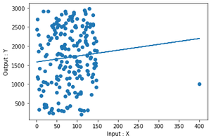
拟合图

步骤4：现在再次拟合回归模型，但是这次我们将删除高杠杆率数据点。

Python3

#Training the regression model with the data that do not
#contain high leverage point
model_nohlp = turicreate.linear_regression.create(
  data_points_with_no_high_leverage_points, target = "Y", features = ["X"])
  
#Plotting the fitted model having no high leverage point
plt.scatter(data_points_with_no_high_leverage_points["X"], 
            data_points_with_no_high_leverage_points["Y"])
plt.xlabel("Input : X")
plt.ylabel("Output : Y")
plt.plot(data_points_with_no_high_leverage_points["X"], 
         model_nohlp.predict(data_points_with_no_high_leverage_points))
plt.show()

输出

拟合图

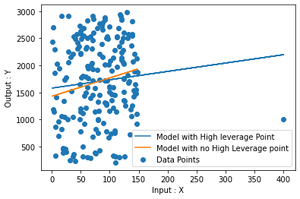
步骤5：到目前为止，您还无法确定两个模型之间的实际差异。因此，让我们将这两个拟合可视化在同一张图片中，以更好地理解它们之间的区别。

Python3

#Plotting both the fitted model in order to compare the results better
plt.scatter(data_points["X"], data_points["Y"], label = "Data Points")
plt.xlabel("Input : X")
plt.ylabel("Output : Y")
  
plt.plot(data_points["X"], model.predict(data_points), 
         label = "Model with High leverage Point")
plt.plot(data_points_with_no_high_leverage_points["X"], 
         model_nohlp.predict(data_points_with_no_high_leverage_points), 
         label = "Model with no High Leverage point")
  
plt.legend()
plt.show()

Python3

#Plotting both the fitted model in order to compare the results better
plt.scatter(data_points["X"], data_points["Y"], label = "Data Points")
plt.xlabel("Input : X")
plt.ylabel("Output : Y")
  
plt.plot(data_points["X"], model.predict(data_points), 
         label="Model with High leverage Point")
  
plt.plot(data_points_with_no_high_leverage_points["X"], 
         model_nohlp.predict(data_points_with_no_high_leverage_points), 
         label = "Model with no High Leverage point")
  
plt.legend()
plt.show()

输出

正如您可以在图中清楚看到的那样，两个图之间的差异仅是通过删除一个点而产生的。

步骤6：现在我们将计算这两个拟合之间的实际差异。为此，我们将计算两个模型的回归系数。

Python3

#Compairing the regression coefficients of both the models
print(f"""
Model with High Leverage Point
{model.coefficients}
-----------------------------------------------------------------------
-----------------------------------------------------------------------
Model without High Leverage Point
{model_nohlp.coefficients}
""")

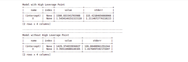
输出

从图片中可以清楚地看出，两个模型的系数之间的差异并不大，但是在实际项目中，实际数据和数据量确实很大，这可能会极大地影响模型的拟合度。但是，分析师仍然需要找出一个数据点是否实际上是高杠杆率，而无需得出任何结论。

在这种情况下，我们使用简单的线性回归来拟合我们的数据，因此我们可以简单地将数据可视化为二维图，但是在多重线性回归的情况下，我们就没有那么奢侈了。在这种情况下，我们必须依靠各种措施来帮助我们确定数据点是否为高杠杆点。