使用机器学习算法的入侵检测系统

问题陈述：任务是构建一个网络入侵检测器，一个能够区分坏连接（称为入侵或攻击）和良好正常连接的预测模型。

介绍：
入侵检测系统是一种使用各种机器学习算法检测网络入侵的软件应用程序。IDS 监视网络或系统的恶意活动，并保护计算机网络免受用户（可能包括内部人员）未经授权的访问。入侵检测器的学习任务是建立一个能够区分“坏连接”（入侵/攻击）和“好（正常）连接”的预测模型（即分类器）。

攻击分为四大类：

• #DOS：拒绝服务，例如syn flood；
• #R2L：来自远程机器的未授权访问，例如猜测密码；
• #U2R：未经授权访问本地超级用户（root）权限，例如各种“缓冲区溢出”攻击；
• #probing：监视和另一个探测，例如端口扫描。

使用的数据集：KDD Cup 1999 数据集

数据集描述：数据文件：

• kddcup.names ：功能列表。
• kddcup.data.gz ：完整的数据集
• kddcup.data_10_percent.gz ：10% 的子集。
• kddcup.newtestdata_10_percent_unlabeled.gz
• kddcup.testdata.unlabeled.gz
• kddcup.testdata.unlabeled_10_percent.gz
• corrected.gz ：使用更正标签测试数据。
• training_attack_types ：入侵类型列表。
• typo-correction.txt ：关于已更正的数据集中的错字的简要说明

特征：

feature name	description	type
duration	length (number of seconds) of the connection	continuous
protocol_type	type of the protocol, e.g. tcp, udp, etc.	discrete
service	network service on the destination, e.g., http, telnet, etc.	discrete
src_bytes	number of data bytes from source to destination	continuous
dst_bytes	number of data bytes from destination to source	continuous
flag	normal or error status of the connection	discrete
land	1 if connection is from/to the same host/port; 0 otherwise	discrete
wrong_fragment	number of “wrong” fragments	continuous
urgent	number of urgent packets	continuous

表 1：单个 TCP 连接的基本特征。

feature name	description	type
hot	number of “hot” indicators	continuous
num_failed_logins	number of failed login attempts	continuous
logged_in	1 if successfully logged in; 0 otherwise	discrete
num_compromised	number of “compromised” conditions	continuous
root_shell	1 if root shell is obtained; 0 otherwise	discrete
su_attempted	1 if “su root” command attempted; 0 otherwise	discrete
num_root	number of “root” accesses	continuous
num_file_creations	number of file creation operations	continuous
num_shells	number of shell prompts	continuous
num_access_files	number of operations on access control files	continuous
num_outbound_cmds	number of outbound commands in an ftp session	continuous
is_hot_login	1 if the login belongs to the “hot” list; 0 otherwise	discrete
is_guest_login	1 if the login is a “guest”login; 0 otherwise	discrete

表 2：领域知识建议的连接中的内容特征。

feature name	description	type
count	number of connections to the same host as the current connection in the past two seconds	continuous
	Note: The following features refer to these same-host connections.
serror_rate	% of connections that have “SYN” errors	continuous
rerror_rate	% of connections that have “REJ” errors	continuous
same_srv_rate	% of connections to the same service	continuous
diff_srv_rate	% of connections to different services	continuous
srv_count	number of connections to the same service as the current connection in the past two seconds	continuous
	Note: The following features refer to these same-service connections.
srv_serror_rate	% of connections that have “SYN” errors	continuous
srv_rerror_rate	% of connections that have “REJ” errors	continuous
srv_diff_host_rate	% of connections to different hosts	continuous

表 3：使用两秒时间窗口计算的交通特征。

应用的各种算法：高斯朴素贝叶斯、决策树、随机森林、支持向量机、逻辑回归。

使用的方法：我在 KDD 数据集上应用了上面提到的各种分类算法，并比较了结果以建立预测模型。

第 1 步 - 数据预处理：

代码：从“kddcup.names”文件导入库和读取功能列表。

import os
import pandas as pd
import numpy as np
import matplotlib.pyplot as plt
import seaborn as sns
import time
  
# reading features list
with open("..\\kddcup.names", 'r') as f:
    print(f.read())

代码：将列附加到数据集并将新列名称“目标”添加到数据集。

cols ="""duration,
protocol_type,
service,
flag,
src_bytes,
dst_bytes,
land,
wrong_fragment,
urgent,
hot,
num_failed_logins,
logged_in,
num_compromised,
root_shell,
su_attempted,
num_root,
num_file_creations,
num_shells,
num_access_files,
num_outbound_cmds,
is_host_login,
is_guest_login,
count,
srv_count,
serror_rate,
srv_serror_rate,
rerror_rate,
srv_rerror_rate,
same_srv_rate,
diff_srv_rate,
srv_diff_host_rate,
dst_host_count,
dst_host_srv_count,
dst_host_same_srv_rate,
dst_host_diff_srv_rate,
dst_host_same_src_port_rate,
dst_host_srv_diff_host_rate,
dst_host_serror_rate,
dst_host_srv_serror_rate,
dst_host_rerror_rate,
dst_host_srv_rerror_rate"""
  
columns =[]
for c in cols.split(', '):
    if(c.strip()):
       columns.append(c.strip())
  
columns.append('target')
print(len(columns))

输出：

42

代码：读取“attack_types”文件。

with open("..\\training_attack_types", 'r') as f:
    print(f.read())

输出：

back dos
buffer_overflow u2r
ftp_write r2l
guess_passwd r2l
imap r2l
ipsweep probe
land dos
loadmodule u2r
multihop r2l
neptune dos
nmap probe
perl u2r
phf r2l
pod dos
portsweep probe
rootkit u2r
satan probe
smurf dos
spy r2l
teardrop dos
warezclient r2l
warezmaster r2l

代码：创建一个攻击类型字典

attacks_types = {
    'normal': 'normal',
'back': 'dos',
'buffer_overflow': 'u2r',
'ftp_write': 'r2l',
'guess_passwd': 'r2l',
'imap': 'r2l',
'ipsweep': 'probe',
'land': 'dos',
'loadmodule': 'u2r',
'multihop': 'r2l',
'neptune': 'dos',
'nmap': 'probe',
'perl': 'u2r',
'phf': 'r2l',
'pod': 'dos',
'portsweep': 'probe',
'rootkit': 'u2r',
'satan': 'probe',
'smurf': 'dos',
'spy': 'r2l',
'teardrop': 'dos',
'warezclient': 'r2l',
'warezmaster': 'r2l',
}

代码：读取数据集（'kddcup.data_10_percent.gz'）并在训练数据集中添加攻击类型特征，其中攻击类型特征有5个不同的值，即dos、normal、probe、r2l、u2r。

path = "..\\kddcup.data_10_percent.gz"
df = pd.read_csv(path, names = columns)
  
# Adding Attack Type column
df['Attack Type'] = df.target.apply(lambda r:attacks_types[r[:-1]])
df.head()
 

代码：数据框的形状和获取每个特征的数据类型

df.shape

输出：

(494021, 43)

代码：查找所有特征的缺失值。

df.isnull().sum()

输出：

duration                       0
protocol_type                  0
service                        0
flag                           0
src_bytes                      0
dst_bytes                      0
land                           0
wrong_fragment                 0
urgent                         0
hot                            0
num_failed_logins              0
logged_in                      0
num_compromised                0
root_shell                     0
su_attempted                   0
num_root                       0
num_file_creations             0
num_shells                     0
num_access_files               0
num_outbound_cmds              0
is_host_login                  0
is_guest_login                 0
count                          0
srv_count                      0
serror_rate                    0
srv_serror_rate                0
rerror_rate                    0
srv_rerror_rate                0
same_srv_rate                  0
diff_srv_rate                  0
srv_diff_host_rate             0
dst_host_count                 0
dst_host_srv_count             0
dst_host_same_srv_rate         0
dst_host_diff_srv_rate         0
dst_host_same_src_port_rate    0
dst_host_srv_diff_host_rate    0
dst_host_serror_rate           0
dst_host_srv_serror_rate       0
dst_host_rerror_rate           0
dst_host_srv_rerror_rate       0
target                         0
Attack Type                    0
dtype: int64

没有找到缺失值，所以我们可以进一步进行下一步。

代码：查找分类特征

# Finding categorical features
num_cols = df._get_numeric_data().columns
  
cate_cols = list(set(df.columns)-set(num_cols))
cate_cols.remove('target')
cate_cols.remove('Attack Type')
  
cate_cols
 

输出：

['service', 'flag', 'protocol_type']

使用条形图可视化分类特征

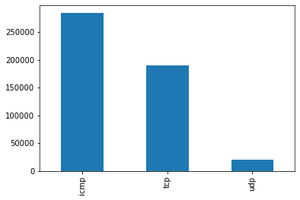
协议类型：我们注意到ICMP在使用的数据中出现最多，然后是TCP和近20000个UDP类型的数据包

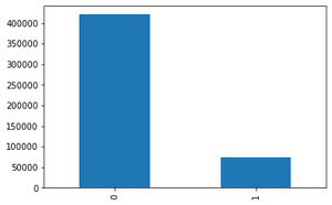
logged_in（如果成功登录则为 1；否则为 0）：我们注意到只有 70000 个数据包成功登录。

目标特征分布：

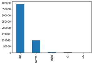
攻击类型（按攻击分组的攻击类型，这是我们将要预测的）

代码：数据相关性——使用热图查找高度相关的变量并忽略它们进行分析。

df = df.dropna('columns')# drop columns with NaN
  
df = df[[col for col in df if df[col].nunique() > 1]]# keep columns where there are more than 1 unique values
  
corr = df.corr()
  
plt.figure(figsize =(15, 12))
  
sns.heatmap(corr)
  
plt.show()
 

输出：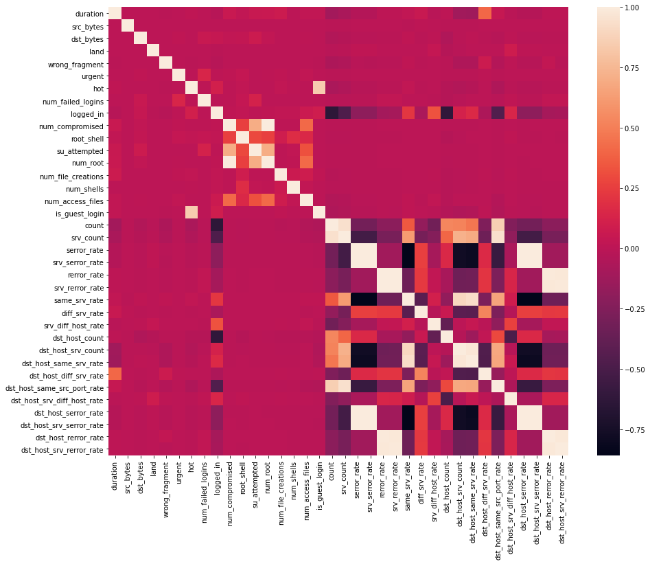

代码：

# This variable is highly correlated with num_compromised and should be ignored for analysis.
#(Correlation = 0.9938277978738366)
df.drop('num_root', axis = 1, inplace = True)
  
# This variable is highly correlated with serror_rate and should be ignored for analysis.
#(Correlation = 0.9983615072725952)
df.drop('srv_serror_rate', axis = 1, inplace = True)
  
# This variable is highly correlated with rerror_rate and should be ignored for analysis.
#(Correlation = 0.9947309539817937)
df.drop('srv_rerror_rate', axis = 1, inplace = True)
  
# This variable is highly correlated with srv_serror_rate and should be ignored for analysis.
#(Correlation = 0.9993041091850098)
df.drop('dst_host_srv_serror_rate', axis = 1, inplace = True)
  
# This variable is highly correlated with rerror_rate and should be ignored for analysis.
#(Correlation = 0.9869947924956001)
df.drop('dst_host_serror_rate', axis = 1, inplace = True)
  
# This variable is highly correlated with srv_rerror_rate and should be ignored for analysis.
#(Correlation = 0.9821663427308375)
df.drop('dst_host_rerror_rate', axis = 1, inplace = True)
  
# This variable is highly correlated with rerror_rate and should be ignored for analysis.
#(Correlation = 0.9851995540751249)
df.drop('dst_host_srv_rerror_rate', axis = 1, inplace = True)
  
# This variable is highly correlated with srv_rerror_rate and should be ignored for analysis.
#(Correlation = 0.9865705438845669)
df.drop('dst_host_same_srv_rate', axis = 1, inplace = True)
 

输出：

代码：特征映射——在特征上应用特征映射，例如：“protocol_type”和“flag”。

# protocol_type feature mapping
pmap = {'icmp':0, 'tcp':1, 'udp':2}
df['protocol_type'] = df['protocol_type'].map(pmap)

代码：

# flag feature mapping
fmap = {'SF':0, 'S0':1, 'REJ':2, 'RSTR':3, 'RSTO':4, 'SH':5, 'S1':6, 'S2':7, 'RSTOS0':8, 'S3':9, 'OTH':10}
df['flag'] = df['flag'].map(fmap)
 

输出：

代码：在建模之前删除不相关的特征，例如“服务”

df.drop('service', axis = 1, inplace = True)

第 2 步 – 建模

代码：导入库并拆分数据集

from sklearn.model_selection import train_test_split
from sklearn.preprocessing import MinMaxScaler
 

代码：

# Splitting the dataset
df = df.drop(['target', ], axis = 1)
print(df.shape)
  
# Target variable and train set
y = df[['Attack Type']]
X = df.drop(['Attack Type', ], axis = 1)
  
sc = MinMaxScaler()
X = sc.fit_transform(X)
  
# Split test and train data 
X_train, X_test, y_train, y_test = train_test_split(X, y, test_size = 0.33, random_state = 42)
print(X_train.shape, X_test.shape)
print(y_train.shape, y_test.shape)
 

输出：

(494021, 31)
(330994, 30) (163027, 30)
(330994, 1) (163027, 1)

应用各种机器学习分类算法，如支持向量机、随机森林、朴素贝叶斯、决策树、逻辑回归来创建不同的模型。

代码：高斯朴素贝叶斯的Python实现

# Gaussian Naive Bayes
from sklearn.naive_bayes import GaussianNB
from sklearn.metrics import accuracy_score
  
clfg = GaussianNB()
start_time = time.time()
clfg.fit(X_train, y_train.values.ravel())
end_time = time.time()
print("Training time: ", end_time-start_time)
 

输出：

Training time:  1.1145250797271729

代码：

start_time = time.time()
y_test_pred = clfg.predict(X_train)
end_time = time.time()
print("Testing time: ", end_time-start_time)
 

输出：

Testing time:  1.543299674987793

代码：

print("Train score is:", clfg.score(X_train, y_train))
print("Test score is:", clfg.score(X_test, y_test))
 

输出：

Train score is: 0.8795114110829804
Test score is: 0.8790384414851528

代码：决策树的Python实现

# Decision Tree 
from sklearn.tree import DecisionTreeClassifier
  
clfd = DecisionTreeClassifier(criterion ="entropy", max_depth = 4)
start_time = time.time()
clfd.fit(X_train, y_train.values.ravel())
end_time = time.time()
print("Training time: ", end_time-start_time)
 

输出：

Training time:  2.4408750534057617

start_time = time.time()
y_test_pred = clfd.predict(X_train)
end_time = time.time()
print("Testing time: ", end_time-start_time)
 

输出：

Testing time:  0.1487727165222168

print("Train score is:", clfd.score(X_train, y_train))
print("Test score is:", clfd.score(X_test, y_test))
 

输出：

Train score is: 0.9905829108684749
Test score is: 0.9905230421954646

代码：随机森林的Python代码实现

from sklearn.ensemble import RandomForestClassifier
  
clfr = RandomForestClassifier(n_estimators = 30)
start_time = time.time()
clfr.fit(X_train, y_train.values.ravel())
end_time = time.time()
print("Training time: ", end_time-start_time)
 

输出：

Training time:  17.084914684295654

start_time = time.time()
y_test_pred = clfr.predict(X_train)
end_time = time.time()
print("Testing time: ", end_time-start_time)
 

输出：

Testing time:  0.1487727165222168

print("Train score is:", clfr.score(X_train, y_train))
print("Test score is:", clfr.score(X_test, y_test))
 

输出：

Train score is: 0.99997583037759
Test score is: 0.9996933023364228

代码：支持向量分类器的Python实现

from sklearn.svm import SVC
  
clfs = SVC(gamma = 'scale')
start_time = time.time()
clfs.fit(X_train, y_train.values.ravel())
end_time = time.time()
print("Training time: ", end_time-start_time)
 

输出：

Training time:  218.26840996742249

代码：

start_time = time.time()
y_test_pred = clfs.predict(X_train)
end_time = time.time()
print("Testing time: ", end_time-start_time)
 

输出：

Testing time:  126.5087513923645

代码：

print("Train score is:", clfs.score(X_train, y_train))
print("Test score is:", clfs.score(X_test, y_test))
 

输出：

Train score is: 0.9987552644458811
Test score is: 0.9987916112055059

代码：逻辑回归的Python实现

from sklearn.linear_model import LogisticRegression
  
clfl = LogisticRegression(max_iter = 1200000)
start_time = time.time()
clfl.fit(X_train, y_train.values.ravel())
end_time = time.time()
print("Training time: ", end_time-start_time)
 

输出：

Training time:  92.94222283363342

代码：

start_time = time.time()
y_test_pred = clfl.predict(X_train)
end_time = time.time()
print("Testing time: ", end_time-start_time)
 

输出：

Testing time:  0.09605908393859863

代码：

print("Train score is:", clfl.score(X_train, y_train))
print("Test score is:", clfl.score(X_test, y_test))
 

输出：

Train score is: 0.9935285835997028
Test score is: 0.9935286792985211

代码：梯度下降的Python实现

from sklearn.ensemble import GradientBoostingClassifier
  
clfg = GradientBoostingClassifier(random_state = 0)
start_time = time.time()
clfg.fit(X_train, y_train.values.ravel())
end_time = time.time()
print("Training time: ", end_time-start_time)
 

输出：

Training time:  633.2290260791779

start_time = time.time()
y_test_pred = clfg.predict(X_train)
end_time = time.time()
print("Testing time: ", end_time-start_time)
 

输出：

Testing time:  2.9503915309906006

print("Train score is:", clfg.score(X_train, y_train))
print("Test score is:", clfg.score(X_test, y_test))
 

输出：

Train score is: 0.9979304760811374
Test score is: 0.9977181693829856

代码：分析每个模型的训练和测试精度。

names = ['NB', 'DT', 'RF', 'SVM', 'LR', 'GB']
values = [87.951, 99.058, 99.997, 99.875, 99.352, 99.793]
f = plt.figure(figsize =(15, 3), num = 10)
plt.subplot(131)
plt.bar(names, values)

输出：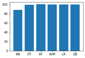

代码：

names = ['NB', 'DT', 'RF', 'SVM', 'LR', 'GB']
values = [87.903, 99.052, 99.969, 99.879, 99.352, 99.771]
f = plt.figure(figsize =(15, 3), num = 10)
plt.subplot(131)
plt.bar(names, values)
 

输出：

代码：分析每个模型的训练和测试时间。

names = ['NB', 'DT', 'RF', 'SVM', 'LR', 'GB']
values = [1.11452, 2.44087, 17.08491, 218.26840, 92.94222, 633.229]
f = plt.figure(figsize =(15, 3), num = 10)
plt.subplot(131)
plt.bar(names, values)
 

输出：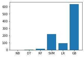

代码：

names = ['NB', 'DT', 'RF', 'SVM', 'LR', 'GB']
values = [1.54329, 0.14877, 0.199471, 126.50875, 0.09605, 2.95039]
f = plt.figure(figsize =(15, 3), num = 10)
plt.subplot(131)
plt.bar(names, values)
 

输出：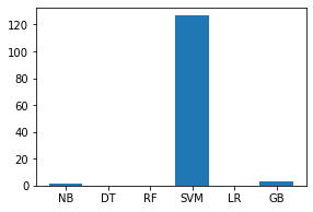

实现链接： https://github.com/mudgalabhay/intrusion-detection-system/blob/master/main.ipynb

结论：以上对不同模型的分析表明，考虑到准确性和时间复杂度，决策树模型最适合我们的数据。

链接：完整代码上传到我的 github 账号上——https://github.com/mudgalabhay/intrusion-detection-system

在评论中写代码？请使用 ide.geeksforgeeks.org，生成链接并在此处分享链接。