Python的量子隐形传态

在本文中，我们将看到使用Python 的量子隐形传态。

瑞克和莫蒂的故事情节有多少次是通过瑞克和莫蒂穿过他们通往某个疯狂的另一个维度的门户开始的？如果不是门户网站，我们可能不会拥有每个人都喜欢的动画电视节目。但是你有没有想过这个门户是如何工作的？这就是我们今天要讲的量子隐形传态。

量子隐形传态需要什么？

除了它会非常棒的事实之外？好吧，正如我们已经知道的，量子计算机与经典计算机并不真正相似。两者之间的差异之一是复制数据。如果您需要复制朋友的作业，您所做的就是单击数据并复制它，对吗？嗯，关于量子位的事情是它们保持在量子状态直到它们不被观察到。一旦我们观察到（或点击）它们，它们就会崩溃到已知状态之一。这也称为不可克隆定理。因此，要在量子计算机上复制数据，我们需要量子隐形传态的过程。然而，随着技术的进步，量子隐形传态已经从这变成了一种完全安全传输的应用程序。

算法背后的理论

为简单起见，我们假设有两个朋友，Kartik 和 Sharanya。 Sharanya 想要向 Kartik 发送某种形式的量子数据，可能是一个量子比特。由于不可克隆定理，她无法观察到量子位的状态，因此她借助所谓的“门户”来传输数据。所以门户的基本作用是，它在来自 Sharanya 的一个量子比特和它自己的一个量子比特之间产生纠缠，并将纠缠对发送到 Kartik。然后，Kartik 必须执行一些操作来消除纠缠并接收输出。

对于那些对什么是量子纠缠不太了解的人，简而言之，它指出，如果一个量子位发生问题，我们可以预期另一个量子位也会产生一些影响，即使这两个量子位彼此相距甚远。此外，另一个有趣的事情要注意为什么这被称为量子传送是 Sharanya 不再拥有与她所做的完全相同的量子位，现在与 Kartik 相同。

方法：

第 1 步：门户创建一对纠缠的 Qubits，这是一个特殊的对，称为 Bell 对。为了使用量子电路创建贝尔对，我们需要取一个量子位并使用 Hadamard 门将其转换为 (|+> 或 |->) 状态，然后在另一个量子位上使用 CNOT 门，这将是由第一个量子位控制。其中一个量子位给 Sharanya（比如 Q1），另一个给 Kartik（比如 Q2）。

第 2 步：假设 Sharanya 想要发送的量子比特是 |Ψ> = |∝> + |β>。她需要对 Q1 应用 CNOT 门，由 |Ψ> 控制。 CNOT 门基本上是量子世界的“如果这个，那么那个”条件。

第 3 步：Sharanya 测量她拥有的两个量子位，并将它们存储在两个经典位中。然后她将此信息发送给 Kartik（由于正在发送经典位，因此可以进行传输）。由于量子位可以处理 2 ^{n 个}经典位，我们可以说 Sharanya 通过她的计算得到的输出将始终是包含 00、01、10 和 11（0 和 1 的所有排列）的概率答案。

第 4 步：现在，Kartik 需要做的就是对他拥有的量子位 Q2 执行某些转换，Q2 是纠缠对的一部分。这部分来自Quantum Mechanics，所以你可以把它当作一个事实，否则文章的复杂性会增加流形。因此，如果 Kartik 得到 00，他需要申请 I 门。对于01，需要应用X门，对于10，需要应用Z门，对于11，需要应用ZX门。

我们终于得到它了。 Kartik 现在的量子位与 Sharanya 最初拥有她的量子位的状态相同。

需要的模块

Qiskit ： Qiskit是一个用于量子计算的开源框架。它提供了用于创建和操作量子程序并在 IBM Q Experience 上的原型量子设备或本地计算机上的模拟器上运行它们的工具。让我们看看如何创建一个简单的 Quantum 电路并在真实的 Quantum 计算机上对其进行测试或在我们的本地计算机中对其进行模拟。

安装：

pip install qiskit

分步实施

第 1 步：创建我们将在其上进行操作的量子电路。

QuantumCircuit 接受 2 个参数，我们想要采用的量子比特数和我们想要采用的经典比特数。

Python

from qiskit import *
  
circuit = QuantumCircuit(3, 3)
%matplotlib inline
  
# Whenever during any point of the program we
# want to see how our circuit looks like,
# this is what we will be doing.
circuit.draw(output='mpl')

输出：

这就是我们的电路现在的样子。我们有 3 个量子位和 3 个经典位，它们将用于随时测量这些量子位的值。现在它们没有任何价值。

第 2 步：在我们必须传送的量子位上应用 X 门。我们还将添加一个屏障，只是为了使电路更清晰。

现在在这里，我们到目前为止所做的是我们有 3 个量子位。我们要做的是使用 q1 将数据从 q0 传输到 q3。为此，我们将使用 X 门将 q0 初始化为 1 状态

Python

circuit.x(0)  # used to apply an X gate.
  
# This is done to make the circuit look more 
# organized and clear.
circuit.barrier()
circuit.draw(output='mpl')

输出：

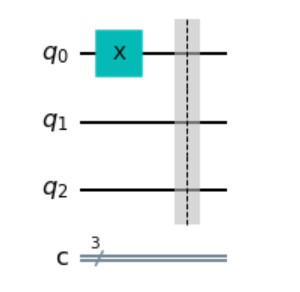
这就是我们的电路现在的样子。在其中一个量子位上，我们添加了一个 X 门，用 X 表示。随着我们不断添加门和其他东西，添加了一个屏障以使电路更有条理。经典位仍然保持不变。

第 3 步：通过在 Q1 上应用 Hadamard 门，在 Q1 和 Q2 上应用 CX 门，在 Q1 和 Q2 之间创建纠缠，从而使 Q1 的行为影响 Q2 的行为。

在这里，我们要做的是创建纠缠，以便第一个量子位的行为影响第二个量子位的行为。

Python

# This is how we apply a Hadamard gate on Q1.
circuit.h(1)
  
# This is the CX gate, which takes two parameters,
# one being the control qubit and the
# other being the target qubit.
circuit.cx(1, 2)
circuit.draw(output='mpl')

输出：

在这里我们可以看到，在这一步之后，这就是我们的电路的样子。我们在 Q1 上应用了一个 Hadamard 门，用“H”符号表示，在 Q1 和 Q2 上有一个受控非（CX）门。经典位仍然保持不变。

通过在 Q0 上应用哈达玛门，在 Q0 和 Q1 上应用 CX 门，在 Q0 和 Q1 之间创建纠缠，从而使 Q1 的行为影响 Q0 的行为。所以本质上，我们有一个系统，其中任何一个量子位的行为都会影响所有量子位的行为。 Q1 可以被视为我们上面谈到的门户。我们现在还将在经典位上投影量子位并测量 Q0 和 Q1 的值。

Python

# The next step is to create a controlled
# gate between qubit 0 and qubit 1.
# Also we will be applying a Hadamard gate to q0.
circuit.cx(0, 1)
circuit.h(0)
  
# Done for clarification of the circuit again.
circuit.barrier()
  
# the next step is to do the two measurements
# on q0 and q1.
circuit.measure([0, 1], [0, 1])
  
# circuit.measure can take any number of arguments,
# and has the following parameters:
# [qubit whos value is to be measured,
# classical bit where the value is stored]
circuit.draw(output='mpl')

输出：

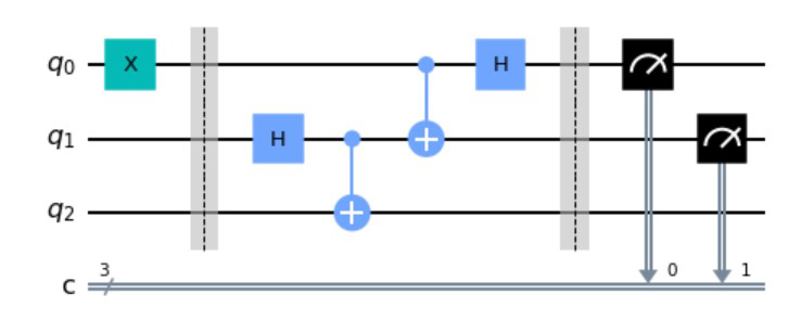
在这里，我们可以看到我们的电路的外观。借助障碍物，您可以轻松区分此步骤中执行的操作。我们在 Q0 上应用了一个 Hadamard 门，用“H”符号表示，在 Q0 和 Q1 上有一个受控非（CX）门。经典位现在投入使用，黑色符号表示我们已取 Q0 和 Q1 的值并将其存储在经典位 1 和经典位 2 中。

实际的解释需要对量子力学的理解，所以人们可以理解，对于经典位的 00 测量，我们需要应用 I 门。对于01，需要应用X门，对于10，需要应用Z门，对于11，需要应用ZX门。由于我们不知道将在经典位中存储什么值，因此我们正在应用更通用的 Control X 门和 Control Z 门。

最后一步是添加两个更多的门，一个受控的 x 门和一个受控的 z 门（我们在上面的文本中已经讨论过这一步，它告诉了哪些门适用于不同的测量）。

Python

circuit.barrier()
circuit.cx(1, 2)
circuit.cz(0, 2)
circuit.draw(output='mpl')

输出：

这是量子隐形传态所需的最终电路。在屏障之后，我们可以看到在 Q1 和 Q2 上应用了受控 X 门，因此 Q2 的行为会影响 Q1 的行为。此外，已应用控制 Z 门，如 Q0 和 Q2 之间所示。

现在我们的电路已经制作完成，我们需要做的就是将该电路传递到模拟器中，以便我们可以从电路中获取结果。一旦我们得到结果，我们就会根据我们收到的经典位的值绘制直方图。您可以将我们现在所做的任何事情视为我们创建的抽象数据类型，下面的代码是我们将使用它的主要函数。每个步骤都进行了完整详细的解释，以方便读者理解。

Python

# The first step is to call a simulator
# which we will use to perform simulations.
from qiskit.tools.visualization import plot_histogram
sim = Aer.get_backend('qasm_simulator')
  
# here, like before, we have given the
# classical bit 2 the value of the Quantum bit 2.
circuit.measure(2, 2)
  
# Now, we run the execute function,
# which takes our quantum circuit,
# the backend which we are using and
# the number of shots we want
# (shots are to increase accuracy and
# mitigate errors in Quantum Computing).
# All of this is stored in a variable called result
  
result = execute(circuit, backend=sim, shots=1000).result()
counts = result.get_counts()
  
# This counts variable shows that for each possible combination,
# how many times the circuit gave a similar output
# (for example, 111 came x times, 101 came y times etc.)
  
# importing plot_histogram which will help us visualize the results.
plot_histogram(counts)

输出：

这如何证明我们的算法有效？

好吧，让我们看看这里。对于 3 个量子位，我们可以有 100、101、111、001 等状态（准确地说，其中 8 个是基本的 P&C 内容）。现在，如果我从 x 轴取一个值，它的读取方式如下：

[100] = [Value stored in classical bit 2, value stored in classical bit 1, value stored in classical bit 0]

我们说过我们将在第二个量子位上的第一个量子位上产生相同的状态。第一个量子比特（Sharanya 拥有的那个（Q0））上的状态是 1，看这里，我们只收到了排列，其中第二个经典比特的值为 1，这证明了第二个量子比特上的值（Kartik 拥有的那个（Q2））也是 1！