使用MATLAB的数字图像处理算法

就像说“一张图片的价值超过一万个单词”一样，数字图像由成千上万个像素组成。

图像也可以定义为二维函数f(x，y)，其中x和y是空间(平面)坐标，因此f在任意一对坐标(x，y)处的振幅称为强度或当时图像的灰度。当x，y以及f的振幅值都是有限的离散量时，我们称该图像为数字图像。

使用各种技术进行图像分割

1.基本过滤器(遮罩)：

以下滤镜用于边缘检测和图像的不连续性。

一阶导数：

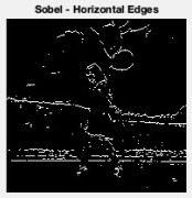
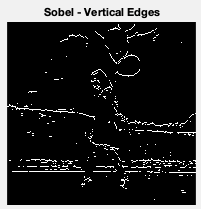
• Sobel遮罩–还用于检测图像中的两种边缘，一种是垂直的，另一种是水平的。
• Prewitt遮罩–它也用于检测图像中的两种类型的边缘：水平边缘和垂直边缘。通过使用图像的相应像素强度之间的差异来计算边缘。
• Robert Mask –通过离散微分来近似图像的梯度，用于边缘检测。

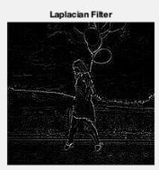
二阶导数运算子：

• 拉普拉斯算子–用于查找图像中快速变化的区域(边缘)。
• LOG (高斯拉普拉斯算子)蒙版(σ= 3)-由于导数滤波器对噪声非常敏感，因此通常在应用拉普拉斯算子之前(使用高斯滤波器)对图像进行平滑处理。此两步过程称为高斯拉普拉斯算子(LoG)操作。
• Canny边缘检测器–这是一种流行的边缘检测算法，它是多阶段的，与其他算法相比，可提供最佳结果。

诸如Prewitt之类的基于梯度的方法具有对噪声敏感的最重要的缺点。 Canny边缘检测器对噪声不太敏感，但比Robert，Sobel和Prewitt贵。但是，Canny边缘检测器的性能优于所有蒙版。

应用Sobel面膜：

输入：

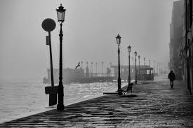
原始图片

代码：

MATLAB

clc;
close all;
clear all;
  
% Read Colour Image and convert it to a grey level Image
% Display the original Image
mycolourimage = imread('image1.jpg');
myimage = rgb2gray(mycolourimage);
subplot(3,3,1); 
imshow(myimage); title('Original Image');
  
% Apply Sobel Operator
% Display only the horizontal Edges
sobelhz = edge(myimage,'sobel','horizontal');
subplot(3,3,2); 
imshow(sobelhz,[]); title('Sobel - Horizontal Edges');
  
% Apply Sobel Operator
% Display only the vertical Edges
sobelvrt = edge(myimage,'sobel','vertical');
subplot(3,3,3); 
imshow(sobelhz,[]); title('Sobel - Vertical Edges');
  
% Apply Sobel Operator
% Display both horizontal and vertical Edges
sobelvrthz = edge(myimage,'sobel','both');
subplot(3,3,4); 
imshow(sobelvrthz,[]); title('Sobel - All edges');

使用MATLAB命令窗口调用上述函数。

输出：

涂Prewitt面膜：

输入：

原始图片

代码：

的MATLAB

clc;
close all;
clear all;
  
% Read Colour Image and convert it to a grey level Image
% Display the original Image
mycolourimage = imread('image1.jpg');
myimage = rgb2gray(mycolourimage);
subplot(3,3,1); 
imshow(myimage); title('Original Image');
  
% Apply Prewitt Operator
% Display both horizontal and vertical Edges
Prewittsedg = edge(myimage,'prewitt');
subplot(3,3,6); 
imshow(Prewittsedg,[]); title('Prewitt - Edges');

使用MATLAB命令窗口调用上述函数。

输出：

应用罗伯特面具：

输入：

原始图片

代码：

的MATLAB

clc;
close all;
clear all;
  
% Read Colour Image and convert it to a grey level Image
% Display the original Image
mycolourimage = imread('image1.jpg');
myimage = rgb2gray(mycolourimage);
subplot(3,3,1); 
imshow(myimage); title('Original Image');
  
% Apply Roberts Operator
% Display both horizontal and vertical Edges
robertsedg = edge(myimage,'roberts');
subplot(3,3,5); 
imshow(robertsedg,[]); title('Roberts - Edges');

使用MATLAB命令窗口调用上述函数。

输出：

涂拉普拉斯面膜：

输入：

原始图片

代码：

的MATLAB

clc;
close all;
clear all;
  
% Read Colour Image and convert it to a grey level Image
% Display the original Image
mycolourimage = imread('image1.jpg');
myimage = rgb2gray(mycolourimage);
subplot(3,3,1); 
imshow(myimage); title('Original Image');
  
% Apply Laplacian Filter   
f=fspecial('laplacian'); 
lapedg = imfilter(myimage,f,'symmetric'); 
subplot(3,3,7); 
imshow(lapedg,[]); title('Laplacian Filter');

使用MATLAB命令窗口调用上述函数。

输出：

应用日志掩码：

输入：

原始图片

代码：

的MATLAB

clc;
close all;
clear all;
  
% Read Colour Image and convert it to a grey level Image
% Display the original Image
mycolourimage = imread('image1.jpg');
myimage = rgb2gray(mycolourimage);
subplot(3,3,1); 
imshow(myimage); title('Original Image');
  
% Apply LOG edge detection  
% The sigma used is 3 
f=fspecial('log',[15,15],3.0);
logedg1 = edge(myimage,'zerocross',[],f);
subplot(3,3,8); 
imshow(logedg1); title('Log with sigma 3');

使用MATLAB命令窗口调用上述函数。

输出：

应用Canny边缘检测器：

输入：

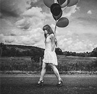
原始图片

代码：

的MATLAB

clc;
close all;
clear all;
  
% Read Colour Image and convert it to a grey level Image
% Display the original Image
mycolourimage = imread('image1.jpg');
myimage = rgb2gray(mycolourimage);
subplot(3,3,1); 
imshow(myimage); title('Original Image');
  
% Apply Canny edge detection   
cannyedg = edge(myimage,'canny');
subplot(3,3,9); 
imshow(cannyedg,[]); title('Canny Edge');

使用MATLAB命令窗口调用上述函数。

输出：

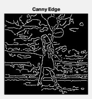
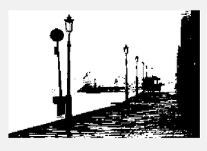
与用于检测图像边缘的其他滤镜/蒙版相比，Canny边缘检测器可提供最佳结果。

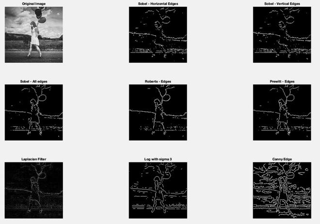
用于边缘检测的所有过滤器的比较

2.环形霍夫变换：

它是霍夫变换的全局处理和专业化。它用于检测输入图像中的圆圈。此变换对圆形具有选择性，并且忽略了细长的椭圆。

输入：

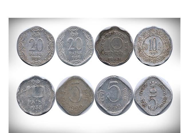
原始图片

代码：

的MATLAB

clc;
close all;
clear all;
  
% Read Colour Image and convert it to a grey level Image
% Display the original Image
% Read the image that have circles
i=imread('image14.jpg');
  
% show image
imshow(i)
  
% select max & min threshold of circles we want to detect
Rmin = 10
Rmax = 50;
  
% Apply Hough circular transform
[centersDark1, radiiDark1] = imfindcircles(i, [Rmin Rmax],'ObjectPolarity','dark','Sensitivity',0.92);
  
% show the detected circles by Red color --
viscircles(centersDark1, radiiDark1,'LineStyle','--')

使用MATLAB命令窗口调用上述函数。

输出：

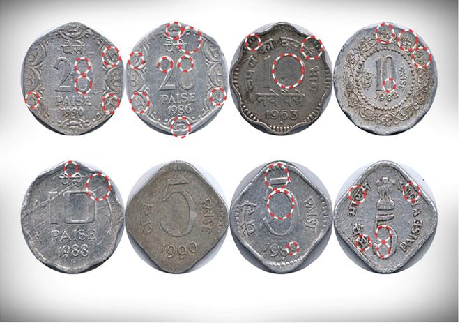
圆形霍夫变换图像

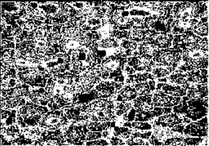
3.阈值选择：

这是一种局部阈值方法，其中我们通过传递一些参数在本地对输入图像进行阈值处理。我们拍摄了已经边缘操作的图像。

输入：

原始图片

代码：

的MATLAB

clc;
close all;
clear all;
  
% Read Colour Image and convert it to a grey level Image
% Display the original Image
image = imread('image2.jpeg');
  
mean_image = imfilter(image, fspecial('average',[15,15]),'replica');
subtract = image - (mean_image+20);
black_white = im2bw(subtract,0);
subplot(1,2,1); imshow(black_white); title('Threshold Image');
subplot(1,2,2); imshow(image); title('Original Image');

使用MATLAB命令窗口调用上述函数。

输出：

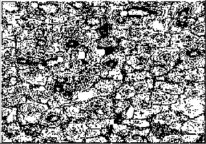
4.大津法：

这是优化全局阈值的一种方法。与本地阈值下的阈值选择相比，Otsu提供最佳结果。该方法使加权的类内方差最小化。

输入：

原始图片

代码：

的MATLAB

clc;
close all;
clear all;
  
% Read Colour Image and convert it to a grey level Image
% Display the original Image
I1=imread('image2.jpeg');
  
%I1=rgb2gray(I);
imshow(I1);
figure, imhist(I1);
T2 = graythresh(I1);
it2= im2bw(I1,T2);
figure,imshow(it2);

使用MATLAB命令窗口调用上述函数。

输出：

全局阈值图像

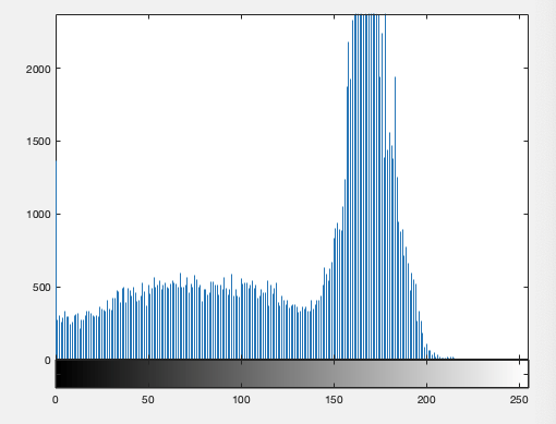
图像直方图

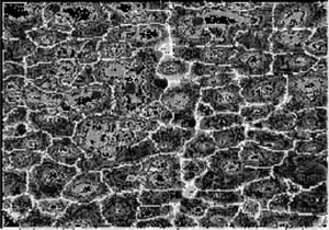
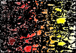
5.形态分水岭：

在此，灰度的局部最小值给出了集水盆地，局部最大值定义了分水岭线。在输出图像中，很容易检测标记。

输入：

原始图片

代码：

的MATLAB

clc;
close all;
clear all;
  
% Read Colour Image and convert it to a grey level Image
% Display the original Image
I= imread('image10.png');
  
%I rgb2gray(RGB);
I1 = imtophat(I, strel('disk', 10));
figure, imshow(I1);
I2 = imadjust(I1);
figure,imshow(I2);
level = graythresh(I2);
BW = im2bw(I2,level);
figure,imshow(BW);
C=~BW;
figure,imshow(C);
D = ~bwdist(C);
D(C) = -Inf;
L = watershed(D);
Wi=label2rgb(L,'hot','w');
figure,imshow(Wi);
im=I;

使用MATLAB命令窗口调用上述函数。

输出：

6. K均值聚类：

它是一种用于从背景中分割兴趣区域的算法。将数据点随机分为K个簇。查找每个群集的质心。

它在2D阵列上运行，其中像素为行，RGB为列。我们为每个类别取平均值(K = 3)。

输入：

原始图片

代码：

的MATLAB

clc;
close all;
clear all;
  
% Read Colour Image and convert it to a grey level Image
  
% Load in an input image
im = imread('image12.png');
  
% We also cast to a double array, because K-means requires it in matlab
imflat = double(reshape(im, size(im,1) * size(im,2), 3));
K = 3
[kIDs, kC] = kmeans(imflat, K, 'Display', 'iter', 'MaxIter', 150, 'Start', 'sample');
colormap = kC / 256;
  
% Scale 0-1, since this is what matlab wants
% Reshape kIDs back into the original image shape
imout = reshape(uint8(kIDs), size(im,1), size(im,2));
imwrite(imout - 1, colormap, 'image6.jpg');

使用MATLAB命令窗口调用上述函数。

输出：

K =
    3
 iter  phase      num          sum
    1      1   178888  1.52491e+08
    2      1     7657  1.45223e+08
    3      1     4597  1.42317e+08
    4      1     3750  1.40017e+08
    5      1     3034  1.38203e+08
    6      1     2187  1.37096e+08
    7      1     1552  1.36481e+08
    8      1     1044  1.36165e+08
    9      1      701  1.36014e+08
   10      1      479  1.35939e+08
   11      1      311  1.35906e+08
   12      1      282  1.35883e+08
   13      1      193   1.3587e+08
   14      1      124  1.35865e+08
   15      1       85  1.35863e+08
   16      1       60  1.35861e+08
   17      1       80   1.3586e+08
   18      1       79  1.35858e+08
   19      1       23  1.35858e+08
   20      1       48  1.35858e+08
   21      1        7  1.35858e+08
Best total sum of distances = 1.35858e+08