Lasso、Ridge 和 Elastic Net 的实现

在本文中，我们将研究不同正则化技术的实现。首先，我们将从多元线性回归开始。为此，我们需要带有 sci-kit learn 和 pandas 预安装的 python3 环境。我们还可以使用 google collaboratory 或任何其他 jupyter notebook 环境。
首先，我们需要将一些包导入到我们的环境中。

Python3

import pandas as pd
import numpy as np
import matplotlib.pyplot as plt
from sklearn import datasets
from sklearn.model_selection import train_test_split
from sklearn.linear_model import LinearRegression

我们将使用波士顿房屋预测数据集。该数据集存在于 sklearn (scikit-learn) 库的数据集模块中。我们可以按如下方式导入此数据集。

Python3

# Loading pre-defined Boston Dataset
boston_dataset = datasets.load_boston()
print(boston_dataset.DESCR)

输出：

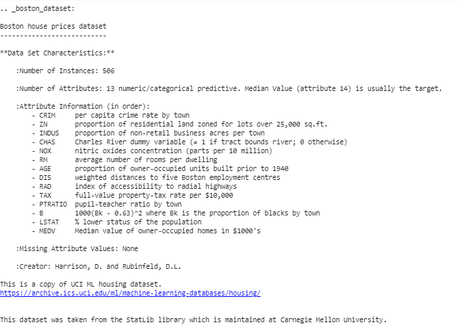
我们可以从上面的描述中得出结论，我们有 13 个自变量和一个因变量（房价）。现在我们需要检查自变量和因变量之间的相关性。我们可以为此使用 scatterplot/corrplot。

Python3

# Generate scatter plot of independent vs Dependent variable
plt.style.use('ggplot')
fig = plt.figure(figsize = (18, 18))
 
for index, feature_name in enumerate(boston_dataset.feature_names):
    ax = fig.add_subplot(4, 4, index + 1)
    ax.scatter(boston_dataset.data[:, index], boston_dataset.target)
    ax.set_ylabel('House Price', size = 12)
    ax.set_xlabel(feature_name, size = 12)
 
plt.show()

上面的代码产生了不同自变量与目标变量的散点图，如下所示

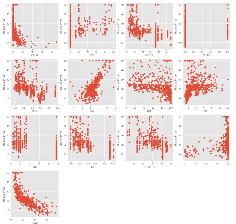
我们可以从上面的散点图中观察到，一些自变量与目标变量的相关性（正或负）不是很大。这些变量将在正则化中降低它们的系数。
代码：用于预处理数据的Python代码。

Python3

# Load the dataset into Pandas Dataframe
boston_pd = pd.DataFrame(boston_dataset.data)
boston_pd.columns = boston_dataset.feature_names
boston_pd_target = np.asarray(boston_dataset.target)
boston_pd['House Price'] = pd.Series(boston_pd_target)
 
# input
X = boston_pd.iloc[:, :-1]
 
#output
Y = boston_pd.iloc[:, -1]
 
print(boston_pd.head())

现在，我们应用训练-测试拆分将数据集分成两部分，一部分用于训练，另一部分用于测试。我们将使用 25% 的数据进行测试。

Python3

x_train, x_test, y_train, y_test = train_test_split(
    boston_pd.iloc[:, :-1], boston_pd.iloc[:, -1],
    test_size = 0.25)
 
print("Train data shape of X = % s and Y = % s : "%(
    x_train.shape, y_train.shape))
 
print("Test data shape of X = % s and Y = % s : "%(
    x_test.shape, y_test.shape))

多元线性回归
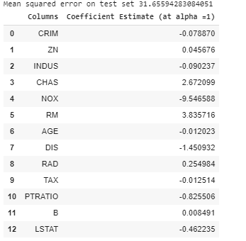
现在是测试模型的正确时机。我们将首先使用多重线性回归。我们在训练数据上训练模型并在测试中计算 MSE。

Python3

# Apply multiple Linear Regression Model
lreg = LinearRegression()
lreg.fit(x_train, y_train)
 
# Generate Prediction on test set
lreg_y_pred = lreg.predict(x_test)
 
# calculating Mean Squared Error (mse)
mean_squared_error = np.mean((lreg_y_pred - y_test)**2)
print("Mean squared Error on test set : ", mean_squared_error)
 
# Putting together the coefficient and their corresponding variable names
lreg_coefficient = pd.DataFrame()
lreg_coefficient["Columns"] = x_train.columns
lreg_coefficient['Coefficient Estimate'] = pd.Series(lreg.coef_)
print(lreg_coefficient)

输出：

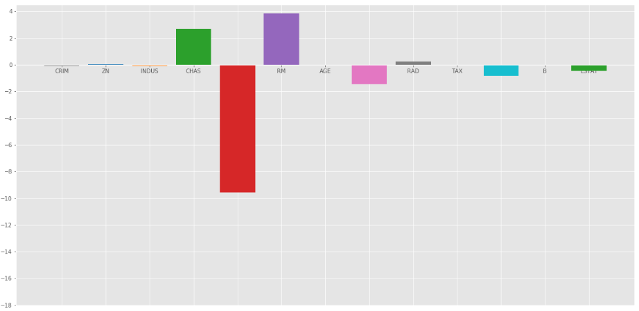
让我们使用 matplotlib 绘图库绘制上述系数的条形图。

Python3

# plotting the coefficient score
fig, ax = plt.subplots(figsize =(20, 10))
 
color =['tab:gray', 'tab:blue', 'tab:orange',
'tab:green', 'tab:red', 'tab:purple', 'tab:brown',
'tab:pink', 'tab:gray', 'tab:olive', 'tab:cyan',
'tab:orange', 'tab:green', 'tab:blue', 'tab:olive']
 
ax.bar(lreg_coefficient["Columns"],
lreg_coefficient['Coefficient Estimate'],
color = color)
 
ax.spines['bottom'].set_position('zero')
 
plt.style.use('ggplot')
plt.show()

输出：

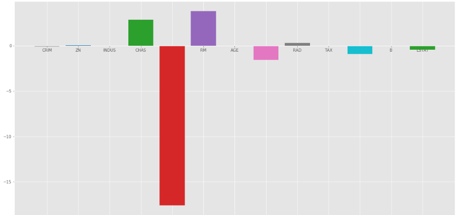
我们可以观察到很多变量的系数都不显着，这些系数对模型的贡献不大，需要调节甚至消除其中的一些变量。岭回归：
Ridge Regression 在普通最小二乘误差函数中添加了一个术语，用于规范变量系数的值。该项是系数乘以参数的平方和。添加此项的目的是惩罚与该系数相对应的变量，该系数与目标变量的相关性不高。该术语称为L ₂正则化。
代码：使用岭回归的Python代码

Python3

# import ridge regression from sklearn library
from sklearn.linear_model import Ridge
 
# Train the model
ridgeR = Ridge(alpha = 1)
ridgeR.fit(x_train, y_train)
y_pred = ridgeR.predict(x_test)
 
# calculate mean square error
mean_squared_error_ridge = np.mean((y_pred - y_test)**2)
print(mean_squared_error_ridge)
 
# get ridge coefficient and print them
ridge_coefficient = pd.DataFrame()
ridge_coefficient["Columns"]= x_train.columns
ridge_coefficient['Coefficient Estimate'] = pd.Series(ridgeR.coef_)
print(ridge_coefficient)

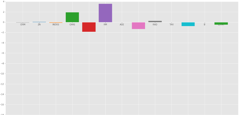
输出： MSE 误差值和带有脊系数的数据帧。

上述数据的条形图为：

岭回归$\alpha$ =1

在上图中，我们取$\alpha$ = 1。
让我们看另一个条形图$\alpha$ = 10

岭回归$\alpha$ = 10

我们可以从上面的图中观察到$\alpha$有助于规范系数并使它们更快地收敛。
请注意，上面的图表可能会产生误导，因为它显示一些系数变为零。在岭正则化中，系数永远不会为 0，它们太小而无法在上面的图中观察到。套索回归：
Lasso 回归类似于 Ridge 回归，除了这里我们添加系数的平均绝对值代替均方值。与岭回归不同，Lasso 回归可以通过将变量的系数值减小到 0 来完全消除变量。我们在普通最小二乘 (OLS) 中添加的新项称为L ₁正则化。
代码：实现套索回归的Python代码

Python3

# import Lasso regression from sklearn library
from sklearn.linear_model import Lasso
 
# Train the model
lasso = Lasso(alpha = 1)
lasso.fit(x_train, y_train)
y_pred1 = lasso.predict(x_test)
 
# Calculate Mean Squared Error
mean_squared_error = np.mean((y_pred1 - y_test)**2)
print("Mean squared error on test set", mean_squared_error)
lasso_coeff = pd.DataFrame()
lasso_coeff["Columns"] = x_train.columns
lasso_coeff['Coefficient Estimate'] = pd.Series(lasso.coef_)
 
print(lasso_coeff)

输出： MSE 误差值和带有 Lasso 系数的数据帧。

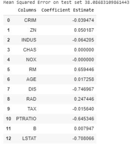
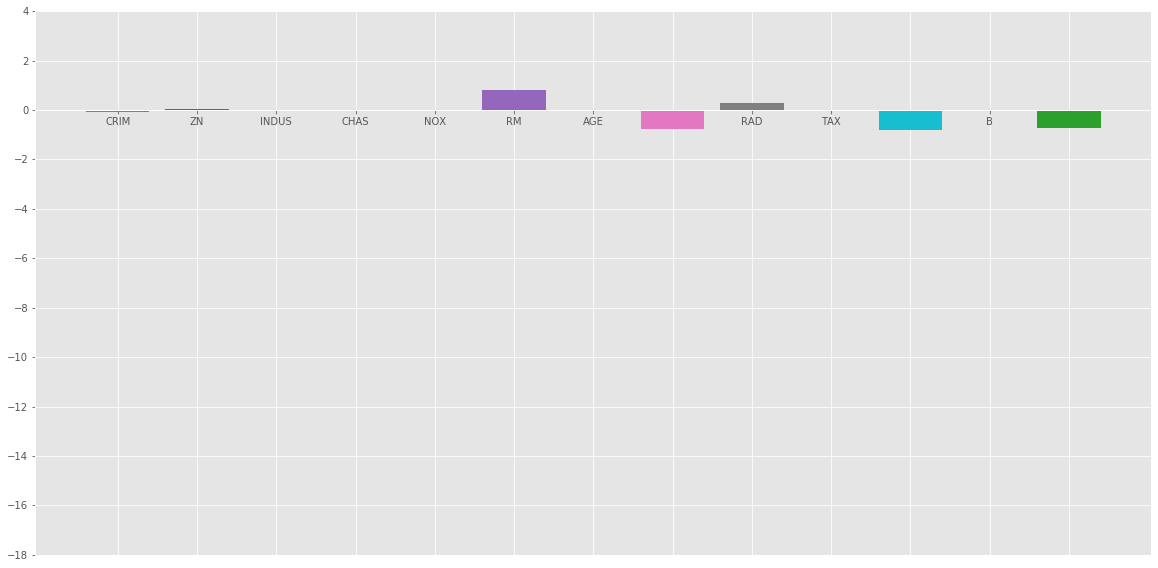
套索回归$\alpha$ = 1

上述系数的条形图：

套索回归$\alpha$ =1

当我们增加$\alpha$ .让我们看看另一个情节$\alpha$ = 10。

弹性网：
在弹性网络正则化中，我们将 L ₁和 L ₂两项相加得到最终的损失函数。这导致我们减少以下损失函数：
$L_{elastic-Net}\left ( \hat\beta \right )= \left ( \sum \left ( y - x_i^J\hat{\beta} \right )^2 \right )/2n+\lambda \left ( (1 -\alpha )/2 * \sum_{j=1}^{m} \hat{\beta_{j}^{2}}+\alpha * \sum_{j=1}^{m} \left \| \hat{\beta_{j}} \right \| \right)$
在哪里$\alpha$介于 0 和 1 之间。当$\alpha$ = 1，它将惩罚项减少到 L ₁惩罚，如果$\alpha$ = 0，它将该项简化为 L ₂
惩罚。
代码：实现弹性网络的Python代码

Python3

# import model
from sklearn.linear_model import ElasticNet
 
# Train the model
e_net = ElasticNet(alpha = 1)
e_net.fit(x_train, y_train)
 
# calculate the prediction and mean square error
y_pred_elastic = e_net.predict(x_test)
mean_squared_error = np.mean((y_pred_elastic - y_test)**2)
print("Mean Squared Error on test set", mean_squared_error)
 
e_net_coeff = pd.DataFrame()
e_net_coeff["Columns"] = x_train.columns
e_net_coeff['Coefficient Estimate'] = pd.Series(e_net.coef_)
e_net_coeff

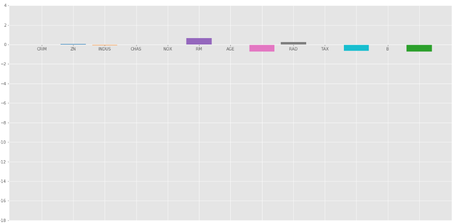
输出：

弹性网

上述系数的条形图：

结论 ：
通过以上分析，我们可以得出以下关于不同正则化方法的结论：

• 正则化用于通过将惩罚项添加到损失函数来减少对任何特定自变量的依赖。该项防止自变量的系数取极值。
  
• 岭回归将 L ₂正则化惩罚项添加到损失函数中。该项减少了系数，但不会使它们为 0，因此不会完全消除任何自变量。它可以用来衡量不同自变量的影响。
  
• Lasso Regression 将 L ₁正则化惩罚项添加到损失函数中。这一项减少了系数，也使它们为0，从而有效地完全消除了相应的自变量。它可以用于特征选择等。
  
• Elastic Net 是上述两种正则化的组合。它包含 L ₁和 L ₂作为其惩罚项。对于大多数测试用例，它的性能优于 Ridge 和 Lasso 回归。