LightGBM vs XGBOOST——哪个算法更好
有很多数据爱好者正在参加机器学习领域的许多在线竞赛。每个人都有自己独特的独立方法来确定最佳模型并预测给定问题陈述的准确输出。在机器学习中,特征工程是整个过程中不可或缺的一部分,也占用了大部分时间。另一方面,建模成为一个重要的部分,你不能有太多的预处理或对特征有一定的限制。有不同的集成方法有助于制作强大的鲁棒模型,这些模型可以提供非常准确的预测。但究竟什么是“合奏”这个词的嗡嗡声?让我们详细了解 Ensemble 一词的含义。
Ensemble:在直接进入技术定义之前,让我们举一个简单的现实生活中的例子并理解相同的内容。让我们假设您想购买一个电子设备——手机。您的第一种方法是在 Internet 上搜索不同的最新智能手机并比较不同公司的费率。您还将看到不同型号的功能。在这第一步之后,您将向您的朋友询问他们对您入围的手机的看法。通过这种方式,您将听取几个人的意见和建议。一旦您获得有关某款手机的一些正面评价,您就会继续购买该手机。这是术语“合奏”的确切概念。集成方法是一种机器学习技术,其中组合了多个基本模型(弱学习器)以生成一个强大的模型。现在让我们更详细地了解 Boosting 方法。
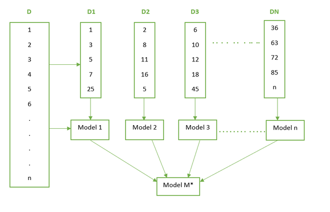
Boosting: Boosting 是 Sequential Ensemble 技术之一。这种技术通常应用于具有高偏差和低方差的数据。这里我们有一个包含 n 条记录的数据集“D”。我们从数据集中随机抽取 5 条记录。这里所有记录被选中的概率相等。因此,通过随机抽样,我们选择了 1、3、5、7、25 条记录。我们在这个样本数据上训练一个模型(让我们说决策树)。之后,我们将 D 数据集的所有记录提供给该模型进行分类。由于模型 1 是一个弱学习器,因此可能会有一些记录被错误分类。错误分类的记录在下一次抽样选择中被赋予更多权重。因此,这些错误分类的记录将比数据集中的其他记录具有更高的选择概率。这里记录 2,8, 1,16 被错误分类,记录 5 也有被选中的概率,所以它被选中了。现在我们再次训练模型 2,然后将完整数据提供给第二个模型。对 n 个模型重复此过程。这些所有模型都是弱学习器。最后,聚合这些模型并构建最终的 M* 模型,该模型是性能更好的模型,因为误分类错误已最小化。下图巧妙地展示了整个过程:
因此,了解了 Boosting 是什么之后,让我们讨论两种流行的 boosting 算法之间的竞争,即 Light Gradient Boosting Machine 和 Extreme Gradient Boosting (xgboost)。这些算法在多个平台上举办的许多比赛和黑客马拉松中取得了最好的结果。现在让我们深入了解算法并对其进行比较研究。
光梯度提升机:
LGBM 是一种快速、分布式、高性能的梯度提升框架,它基于流行的机器学习算法——决策树。它可用于分类、回归和更多机器学习任务。该算法以叶方式增长,并选择最大的增量值进行增长。 LightGBM 使用基于直方图的算法。这样做的优点如下:
- 更少的内存使用
- 减少并行学习的通信成本
- 降低用于计算决策树中每个拆分的增益的成本。
因此,随着 LightGBM 的训练速度更快,但有时也会导致过度拟合的情况。那么,让我们看看可以调整哪些参数以获得更好的最优模型。
要获得最佳拟合,必须调整以下参数:
- num_leaves:由于 LightGBM 以叶方式增长,因此该值必须小于 2^(max_depth) 以避免过度拟合的情况。
- min_data_in_leaf:对于大型数据集,其值应设置为数百到数千。
- max_depth:一个关键参数,其值应相应设置以避免过度拟合。
为了获得更好的精度,必须调整以下参数:
- 添加到模型中的更多训练数据可以提高准确性。 (也可以是外部看不见的数据)
- num_leaves:增加它的值会提高精度,因为分裂是按叶进行的,但也可能发生过拟合。
- max_bin:高值会对准确率产生重大影响,但最终会过度拟合。
XGBOOST 算法:
一种非常流行和需求的算法,通常被称为不同平台上各种比赛的获胜算法。 XGBOOST 代表极限梯度提升。该算法是梯度提升算法的改进版本。基本算法是梯度提升决策树算法。其强大的预测能力和易于实施的方法使其在许多机器学习笔记本中无处不在。该算法的一些关键点如下:
- 它不会构建完整的树结构,而是贪婪地构建它。
- 与 LightGBM 相比,它是按级别拆分而不是按叶拆分。
- 在梯度提升中,考虑负梯度来优化损失函数,但这里考虑了泰勒展开。
- 正则化项会惩罚构建复杂的树模型。
一些可以调整以提高性能的参数如下:
一般参数包括以下内容:
- booster:它有 2 个选项—— gbtree和gblinear 。
- 静默:如果保持为 1,则在代码执行时不会显示正在运行的消息。
- nthread:主要用于并行处理。此处指定内核数。
助推器参数包括以下内容:
- eta:通过在每一步缩小权重来使模型健壮。
- max_depth:应相应设置以避免过度拟合。
- max_leaf_nodes:如果定义了这个参数,那么模型将忽略max_depth 。
- gamma:指定进行拆分所需的最小损失减少。
- lambda:权重上的 L2 正则化项。
学习任务参数包括以下内容:
1)目标:这将定义要使用的损失函数。
- 二元:用于二元分类的逻辑 - 逻辑回归,返回预测概率(不是类)
- multi: softmax – 使用 softmax 目标的多类分类,返回预测类(不是概率)
2)种子:为此设置的默认值为零。可用于参数调整。
因此,我们已经了解了算法的基础知识以及需要针对相应算法进行调整的参数。现在我们将获取一个数据集,然后根据准确性和执行时间比较这两种算法。下面是我们将要使用的数据集描述:
数据集描述:
这些实验是在 19-48 岁年龄段的 30 名志愿者中进行的。每个人在腰部佩戴智能手机(三星 Galaxy S II)进行六项活动(WALKING、WALKING_UPSTAIRS、WALKING_DOWNSTAIRS、SITTING、STANDING、LAYING)。使用其嵌入式加速度计和陀螺仪,我们以 50Hz 的恒定速率捕获了 3 轴线性加速度和 3 轴角速度。实验已被录像以手动标记数据。将获得的数据集随机分为两组,其中 70% 的志愿者被选中用于生成训练数据,30% 的志愿者被选中用于测试数据。
传感器信号(加速度计和陀螺仪)通过应用噪声滤波器进行预处理,然后在 2.56 秒和 50% 重叠(128 个读数/窗口)的固定宽度滑动窗口中采样。传感器加速度信号具有重力和身体运动分量,使用巴特沃斯低通滤波器将其分离为身体加速度和重力。假设重力只有低频分量,因此使用了截止频率为 0.3 Hz 的滤波器。从每个窗口,通过计算来自时域和频域的变量来获得特征向量。
数据链接: https://github.com/pranavkotak8/Datasets/blob/master/smartphone_activity_dataset.zip
Python代码实现:
Python3
# Importing the basic libraries
pip install pandas
import time
import pandas as pd
import numpy as np
import seaborn as sns
import matplotlib.pyplot as plt
%matplotlib inline
import gc

gc.enable()

# Importing LGBM and XGBOOST
import lightgbm as lgb
import xgboost as xgb

# Reading the Data and Inspecting it
data=pd.read_csv('/content/drive/MyDrive/GeeksforGeeks_Datasets/smartphone_activity_dataset.csv')
data
Python3
# Checking for missing values across the 562 features of the dataset
data.isna().sum()*100/len(data)

# Checking for Target Distribution
sns.countplot(data['activity'])
plt.show()
Python3
# Saving the target variable(dependent variable) to target
# variable and dropping it from the original "data" dataframe
target=data['activity']
data.drop(columns={'activity'},inplace=True)

# As the dataset contains all numerical features and also
# the target classes are also encoded there is no more preprocessing
# needed at this stage. There are no missing values in the
# dataset hence no missing data imputation is being needed.
# Let us split the dataset and move to the modeling part.

# Splitting the Dataset into Training and Testing Dataset
from sklearn.model_selection import train_test_split
X_train,X_test,y_train,y_test=train_test_split(
  data,target,test_size=0.15,random_state=100)

# Applying the XGBOOST Model
# Setting Parameters required for XGBOOST Model
# and Training the Model

# Starting to track the Time
start = time.time()
xg=xgb.XGBClassifier(max_depth=7,learning_rate=0.05,
                     silent=1,eta=1,objective='multi:softprob',
                     num_round=50,num_classes=6)

# Setting the Parameters. More parameters can be set
# according to the requirement.
# Here we have set the main parameters.

# Fitting the Model
xg.fit(X_train,y_train)

# Stopping the tracking of time
stop = time.time()
exec_time_xgb=stop-start

# Measuring the time taken for the model to build
exec_time_xgb

# Predicting the Output Class
ypred_xgb=xg.predict(X_test)
ypred_xgb


# Getting the Accuracy Score for the XGBOOST Model
from sklearn.metrics import accuracy_score
accuracy_xgb = accuracy_score(y_test,ypred_xgb)

# Setting the Parameters and Training data for LightGBM Model
data_train = lgb.Dataset(X_train,label = y_train)
params= {}

# Usually set between 0 to 1.
params['learning_rate']=0.5

# GradientBoostingDecisionTree
params['boosting_type']='gbdt'

# Multi-class since the target class has 6 classes.
params['objective']='multiclass'

# Metric for multi-class
params['metric']='multi_logloss'
params['max_depth']=7
params['num_class']=7

# This value is not inclusive of the end value.
# Hence we have 6 classes the value is set to 7.

# Training the LightGBM Model
num_round =50
start = time.time()
lgbm = lgb.train(params,data_train,num_round)
stop = time.time()

#Execution time of the LightGBM Model
exec_time_lgbm = stop-start
exec_time_lgbm

# Predicting the output on the Test Dataset
ypred_lgbm = lgbm.predict(X_test)
ypred_lgbm
y_pred_lgbm_class = [np.argmax(line) for line in ypred_lgbm]
Python3
# Accuracy Score for the LightGBM Model
from sklearn.metrics import accuracy_score
accuracy_lgbm=accuracy_score(y_test,y_pred_lgbm_class)
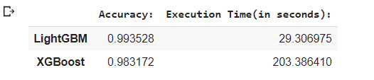
# Comparing the Accuracy and Execution Time for both the Algorithms
comparison = {'Accuracy:':(accuracy_lgbm,accuracy_xgb),\
'Execution Time(in seconds):':(exec_time_lgbm,exec_time_xgb)}
LGBM_XGB = pd.DataFrame(comparison)
LGBM_XGB .index = ['LightGBM','XGBoost']
LGBM_XGB
# On comparison we notice that LightGBM is
# faster and gives better accuracy.
comp_ratio=(203.594708/29.443264)
comp_ratio
print("LightGBM is "+" "+str(np.ceil(comp_ratio))+" "+\
str("times")+" "+"faster than XGBOOST Algorithm")蟒蛇3
# Checking for missing values across the 562 features of the dataset
data.isna().sum()*100/len(data)

# Checking for Target Distribution
sns.countplot(data['activity'])
plt.show()
蟒蛇3
# Saving the target variable(dependent variable) to target
# variable and dropping it from the original "data" dataframe
target=data['activity']
data.drop(columns={'activity'},inplace=True)

# As the dataset contains all numerical features and also
# the target classes are also encoded there is no more preprocessing
# needed at this stage. There are no missing values in the
# dataset hence no missing data imputation is being needed.
# Let us split the dataset and move to the modeling part.

# Splitting the Dataset into Training and Testing Dataset
from sklearn.model_selection import train_test_split
X_train,X_test,y_train,y_test=train_test_split(
  data,target,test_size=0.15,random_state=100)

# Applying the XGBOOST Model
# Setting Parameters required for XGBOOST Model
# and Training the Model

# Starting to track the Time
start = time.time()
xg=xgb.XGBClassifier(max_depth=7,learning_rate=0.05,
                     silent=1,eta=1,objective='multi:softprob',
                     num_round=50,num_classes=6)

# Setting the Parameters. More parameters can be set
# according to the requirement.
# Here we have set the main parameters.

# Fitting the Model
xg.fit(X_train,y_train)

# Stopping the tracking of time
stop = time.time()
exec_time_xgb=stop-start

# Measuring the time taken for the model to build
exec_time_xgb

# Predicting the Output Class
ypred_xgb=xg.predict(X_test)
ypred_xgb


# Getting the Accuracy Score for the XGBOOST Model
from sklearn.metrics import accuracy_score
accuracy_xgb = accuracy_score(y_test,ypred_xgb)

# Setting the Parameters and Training data for LightGBM Model
data_train = lgb.Dataset(X_train,label = y_train)
params= {}

# Usually set between 0 to 1.
params['learning_rate']=0.5

# GradientBoostingDecisionTree
params['boosting_type']='gbdt'

# Multi-class since the target class has 6 classes.
params['objective']='multiclass'

# Metric for multi-class
params['metric']='multi_logloss'
params['max_depth']=7
params['num_class']=7

# This value is not inclusive of the end value.
# Hence we have 6 classes the value is set to 7.

# Training the LightGBM Model
num_round =50
start = time.time()
lgbm = lgb.train(params,data_train,num_round)
stop = time.time()

#Execution time of the LightGBM Model
exec_time_lgbm = stop-start
exec_time_lgbm

# Predicting the output on the Test Dataset
ypred_lgbm = lgbm.predict(X_test)
ypred_lgbm
y_pred_lgbm_class = [np.argmax(line) for line in ypred_lgbm]
蟒蛇3
# Accuracy Score for the LightGBM Model
from sklearn.metrics import accuracy_score
accuracy_lgbm=accuracy_score(y_test,y_pred_lgbm_class)

# Comparing the Accuracy and Execution Time for both the Algorithms
comparison = {'Accuracy:':(accuracy_lgbm,accuracy_xgb),\
              'Execution Time(in seconds):':(exec_time_lgbm,exec_time_xgb)}
LGBM_XGB = pd.DataFrame(comparison)
LGBM_XGB .index = ['LightGBM','XGBoost']
LGBM_XGB

# On comparison we notice that LightGBM is
# faster and gives better accuracy.
comp_ratio=(203.594708/29.443264)
comp_ratio
print("LightGBM is "+" "+str(np.ceil(comp_ratio))+" "+\
      str("times")+" "+"faster than XGBOOST Algorithm")
最终输出: