人类活动识别——使用深度学习模型

使用诸如加速度计等智能手机传感器的人类活动识别是研究的热点之一。 HAR 是时间序列分类问题之一。在这个项目中，已经制定了各种机器学习和深度学习模型，以获得最佳的最终结果。在相同的序列中，我们可以使用循环神经网络（RNN）的 LSTM（长短期记忆）模型来识别人类的各种活动，如站立、爬楼和爬楼等。
LSTM 模型是一种递归神经网络，能够学习序列预测问题中的顺序依赖性。使用此模型是因为这有助于记住任意间隔内的值。
人类活动识别数据集可以从下面给出的链接下载：HAR 数据集
活动：

• 步行
• 楼上
• 楼下
• 坐着
• 常设

加速度计检测适当加速度的大小和方向，作为矢量，并可用于感知方向（因为重量方向发生变化）。根据角动量守恒，陀螺仪保持沿轴的方向，以便方向不受支架倾斜或旋转的影响。
了解数据集：

• 随着时间的推移，这两个传感器都会在 3D 空间中生成数据。
  （“XYZ”表示 X、Y 和 Z 方向的 3 轴信号。）
• 可用数据通过应用噪声滤波器进行预处理，然后在固定宽度的窗口中进行采样，即每个窗口有 128 个读数。

训练和测试数据被分开为
80% 志愿者的读数作为训练数据，其余 20% 志愿者的记录作为测试数据。所有数据都存在于使用上面提供的链接下载的文件夹中。
阶段

• 选择数据集
  
• 上传驱动器中的数据集以在 google colaboratory 上工作
• 数据集清洗和数据预处理
• 选择模型并构建深度学习网络模型
• 在 Android Studio 中导出。

该项目使用的 IDE 是 Google Colaboratory，这是处理深度学习项目的最佳时代。第 1 阶段已在上面解释为从哪里下载数据集。按照这个顺序开始项目，在 Google Colaboratory 中打开一个新笔记本，首先导入所有必要的库。
代码：导入库

Python3

import pandas as pd
import numpy as np
import pickle
import matplotlib.pyplot as plt
from scipy import stats
import tensorflow as tf
import seaborn as sns
from sklearn import metrics
from sklearn.model_selection import train_test_split
 
%matplotlib inline

阶段2：
它正在将数据集上传到笔记本中，在此之前我们需要将笔记本安装在驱动器上，以便将此笔记本保存在我们的驱动器上并在需要时检索。

Python3

sns.set(style="whitegrid", palette="muted", font_scale=1.5)
RANDOM_SEED = 42
 
from google.colab import drive
drive.mount('/content/drive')

输出：

You will see a pop up similar to one shown in the screenshot below, open the link and copy the authorization code and paste it in the authorization code bar and enter the drive will be mounted.

代码：上传数据集

Python3

from google.colab import files
uploaded = files.upload()

现在进入模型构建和训练阶段，我们需要寻找不同的模型来帮助构建更准确的模型。这里，选择了循环神经网络的 LSTM 模型。下面给出的图像显示了数据的外观。

第三阶段：
它从数据预处理开始。在这个阶段，大约 90% 的时间都花在了实际的数据科学项目中。在这里，原始数据被获取并转换为一些有用且有效的格式。
代码：执行数据转换以规范化数据

Python3

#transforming shape
reshaped_segments = np.asarray(
    segments, dtype = np.float32).reshape(
    -1 , N_time_steps, N_features)
 
reshaped_segments.shape

代码：拆分数据集

Python3

X_train, X_test, Y_train, Y_test = train_test_split(
    reshaped_segments, labels, test_size = 0.2,
    random_state = RANDOM_SEED)

测试规模取为 20%，即总记录中 20% 的记录用于测试准确性，其余记录用于训练模型。
班级数 = 6（走、坐、站、跑、楼上和楼下）
第 4 阶段：在此阶段模型中选择的是 RNN 的 LSTM 模型。
代码：模型构建

Python3

def create_LSTM_model(inputs):
    W = {
        'hidden': tf.Variable(tf.random_normal([N_features, N_hidden_units])),
        'output': tf.Variable(tf.random_normal([N_hidden_units, N_classes]))
    }
    biases = {
        'hidden': tf.Variable(tf.random_normal([N_hidden_units], mean = 0.1)),
        'output': tf.Variable(tf.random_normal([N_classes]))
    }
    X = tf.transpose(inputs, [1, 0, 2])
    X = tf.reshape(X, [-1, N_features])
    hidden = tf.nn.relu(tf.matmul(X, W['hidden']) + biases['hidden'])
    hidden = tf.split(hidden, N_time_steps, 0)
 
    lstm_layers = [tf.contrib.rnn.BasicLSTMCell(
        N_hidden_units, forget_bias = 1.0) for _ in range(2)]
    lstm_layers = tf.contrib.rnn.MultiRNNCell(lstm_layers)
 
    outputs, _ = tf.contrib.rnn.static_rnn(lstm_layers,
                                           hidden, dtype = tf.float32)
 
    lstm_last_output = outputs[-1]
    return tf.matmul(lstm_last_output, W['output']) + biases['output']

代码：使用 AdamOptimizer 执行优化以修改变量的损失值，以提高准确性并减少损失。

Python3

L2_LOSS = 0.0015
l2 = L2_LOSS * \
  sum(tf.nn.l2_loss(tf_var) for tf_var in tf.trainable_variables())
loss = tf.reduce_mean(tf.nn.softmax_cross_entropy_with_logits(
    logits = pred_y, labels = Y)) + l2
 
Learning_rate = 0.0025
optimizer = tf.train.AdamOptimizer(learning_rate = Learning_rate).minimize(loss)
correct_pred = tf.equal(tf.argmax(pred_softmax , 1), tf.argmax(Y,1))
accuracy = tf.reduce_mean(tf.cast(correct_pred, dtype = tf.float32))

代码：执行 50 次模型训练迭代以获得最高准确率并减少损失

Python3

# epochs is number of iterations performed in model training.
N_epochs = 50 
batch_size = 1024
 
saver = tf.train.Saver()
history = dict(train_loss=[], train_acc=[], test_loss=[], test_acc=[])
sess = tf.InteractiveSession()
sess.run(tf.global_variables_initializer())
train_count = len(X_train)
 
for i in range(1, N_epochs + 1):
    for start, end in zip(range(0, train_count, batch_size),
                          range(batch_size, train_count + 1, batch_size)):
        sess.run(optimizer, feed_dict={X: X_train[start:end],
                                       Y: Y_train[start:end]})
    _, acc_train, loss_train = sess.run([pred_softmax, accuracy, loss], feed_dict={
        X: X_train, Y: Y_train})
    _, acc_test, loss_test = sess.run([pred_softmax, accuracy, loss], feed_dict={
        X: X_test, Y: Y_test})
    history['train_loss'].append(loss_train)
    history['train_acc'].append(acc_train)
    history['test_loss'].append(loss_test)
    history['test_acc'].append(acc_test)
 
    if (i != 1 and i % 10 != 0):
        print(f'epoch: {i} test_accuracy:{acc_test} loss:{loss_test}')
predictions, acc_final, loss_final = sess.run([pred_softmax, accuracy, loss],
                                              feed_dict={X: X_test, Y: Y_test})
print()
print(f'final results : accuracy : {acc_final} loss : {loss_final}')
    

输出：

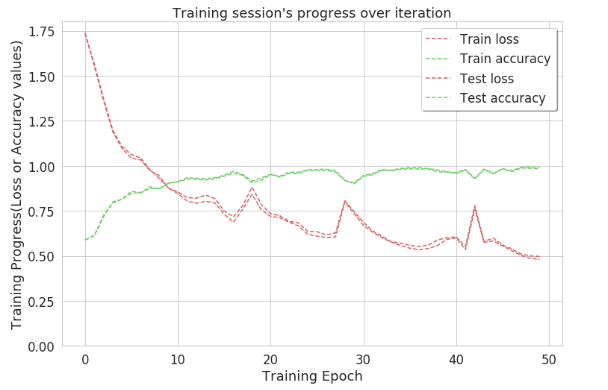
因此，使用这种方法，在第 50 次迭代时，准确率接近 1。这表明通过这种方法可以清楚地识别大多数标签。为了获得正确识别的活动的准确计数，创建了混淆矩阵。
代码：精度图

Python3

plt.figure(figsize=(12,8))
 
plt.plot(np.array(history['train_loss']), "r--", label="Train loss")
plt.plot(np.array(history['train_acc']), "g--", label="Train accuracy")
 
plt.plot(np.array(history['test_loss']), "r--", label="Test loss")
plt.plot(np.array(history['test_acc']), "g--", label="Test accuracy")
 
plt.title("Training session's progress over iteration")
plt.legend(loc = 'upper right', shadow = True)
plt.ylabel('Training Progress(Loss or Accuracy values)')
plt.xlabel('Training Epoch')
plt.ylim(0)
 
plt.show()

混淆矩阵：混淆矩阵不亚于二维矩阵，不像它有助于计算正确识别的活动的精确计数。换句话说，它描述了分类模型在测试数据集上的性能。
代码：混淆矩阵

Python3

max_test = np.argmax(Y_test, axis=1)
max_predictions = np.argmax(predictions, axis = 1)
confusion_matrix = metrics.confusion_matrix(max_test, max_predictions)
 
plt.figure(figsize=(16,14))
sns.heatmap(confusion_matrix, xticklabels = LABELS, yticklabels = LABELS, annot =True, fmt = "d")
plt.title("Confusion Matrix")
plt.xlabel('Predicted_label')
plt.ylabel('True Label')
plt.show()

这是迄今为止有关该项目的完整描述。它可以使用其他模型（如 CNN）或机器学习模型（如 KNN）来构建。