在 R 编程中使用相关图可视化相关矩阵

相关矩阵的图称为Correlogram 。这通常用于突出显示数据集或数据表中最相关的变量。图中的相关系数根据值着色。根据变量之间的关联程度，我们可以对相关矩阵进行相应的重新排序。

R中的相关图

在 R 中，我们将使用“corrplot”包来实现相关图。因此，要从 R 控制台安装软件包，我们应该执行以下命令：

install.packages("corrplot")

一旦我们正确安装了包，我们将使用library()函数在我们的 R 脚本中加载包，如下所示：

library("corrplot")

我们现在将看到如何在 R 编程中实现相关图。我们将通过一个例子一步一步地看到实现的详细解释。

例子：

第 1 步：[用于相关分析的数据]：第一项工作是选择合适的数据集来实现该概念。对于我们的示例，我们将使用“mtcars”数据集，它是 R 的内置数据集。我们将看到该数据集中的一些数据。

R

# Correlogram in R
# including the required packages
library(corrplot)
  
head(mtcars)

输出：

head(mtcars)
                   mpg cyl disp  hp drat    wt  qsec vs am gear carb
Mazda RX4         21.0   6  160 110 3.90 2.620 16.46  0  1    4    4
Mazda RX4 Wag     21.0   6  160 110 3.90 2.875 17.02  0  1    4    4
Datsun 710        22.8   4  108  93 3.85 2.320 18.61  1  1    4    1
Hornet 4 Drive    21.4   6  258 110 3.08 3.215 19.44  1  0    3    1
Hornet Sportabout 18.7   8  360 175 3.15 3.440 17.02  0  0    3    2
Valiant           18.1   6  225 105 2.76 3.460 20.22  1  0    3    1

第 2 步：[计算相关矩阵]：我们现在将计算一个相关矩阵，我们要为其绘制相关图。我们将使用cor()函数来计算相关矩阵。

R

# Correlogram in R
# required packages
library(corrplot)
  
head(mtcars)
#correlation matrix
M<-cor(mtcars)
head(round(M,2))

输出：

head(round(M,2))
       mpg   cyl  disp    hp  drat    wt  qsec    vs    am  gear  carb
mpg   1.00 -0.85 -0.85 -0.78  0.68 -0.87  0.42  0.66  0.60  0.48 -0.55
cyl  -0.85  1.00  0.90  0.83 -0.70  0.78 -0.59 -0.81 -0.52 -0.49  0.53
disp -0.85  0.90  1.00  0.79 -0.71  0.89 -0.43 -0.71 -0.59 -0.56  0.39
hp   -0.78  0.83  0.79  1.00 -0.45  0.66 -0.71 -0.72 -0.24 -0.13  0.75
drat  0.68 -0.70 -0.71 -0.45  1.00 -0.71  0.09  0.44  0.71  0.70 -0.09
wt   -0.87  0.78  0.89  0.66 -0.71  1.00 -0.17 -0.55 -0.69 -0.58  0.43

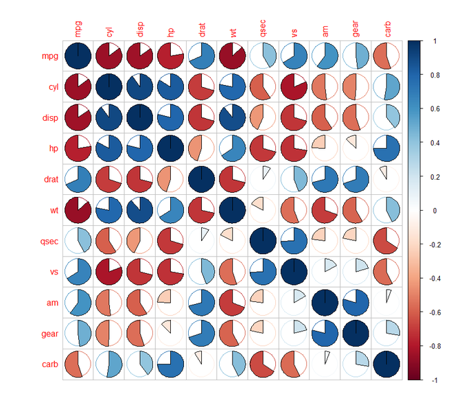
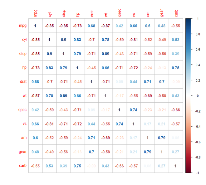
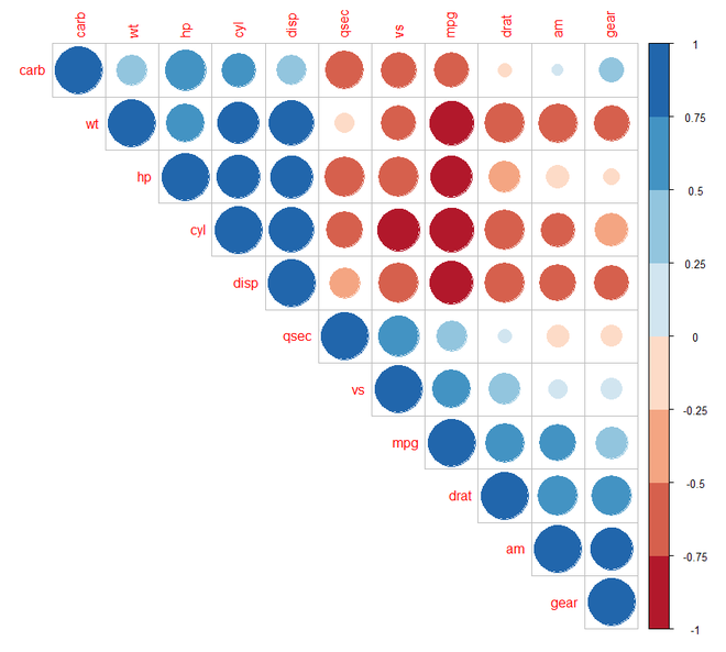
第 3 步：[使用方法参数可视化]：首先，我们将了解如何将相关图可视化为不同形状，如圆形、饼形、椭圆形等。我们将使用corrplot()函数并在其方法参数中提及形状。

R

# Correlogram in R
# required packages
library(corrplot)
  
head(mtcars)
#correlation matrix
M<-cor(mtcars)
head(round(M,2))
  
#visualizing correlogram
#as circle
corrplot(M, method="circle")
# as pie
corrplot(M, method="pie")
# as colour
corrplot(M, method="color")
# as number
corrplot(M, method="number")

输出：

第 4 步：[使用类型参数可视化]：我们将了解如何可视化不同类型的相关图，例如上三角矩阵和下三角矩阵。我们将使用corrplot()函数并提及类型参数。

R

# Correlogram in R
# required package
library(corrplot)
  
head(mtcars)
  
# correlation matrix
M<-cor(mtcars)
head(round(M,2))
  
# types
# upper triangular matrix
corrplot(M, type="upper")
  
# lower triangular matrix
corrplot(M, type="lower")

输出：

第 5 步：[重新排序相关图]：我们将了解如何重新排序相关图。我们将使用corrplot()函数并提及order 参数。我们将使用“hclust”排序进行层次聚类。

R

# Correlogram in R
# required packages
library(corrplot)
  
head(mtcars)
  
# correlation matrix
M<-cor(mtcars)
head(round(M, 2))
  
# reordering
# correlogram with hclust reordering
corrplot(M, type = "upper", order = "hclust")
  
# Using different color spectrum
col<- colorRampPalette(c("red", "white", "blue"))(20)
corrplot(M, type="upper", order = "hclust", col = col)
  
# Change background color to lightblue
corrplot(M, type="upper", order="hclust", 
         col = c("black", "white"), 
         bg = "lightblue")

输出：

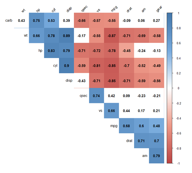
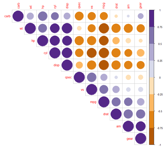
第 6 步：[更改相关图中的颜色]：现在我们将了解如何更改相关图中的颜色。为此，我们安装了“RColorBrewer”包并将其添加到我们的 R 脚本中以使用其调色板颜色。

R

# Correlogram in R
# required package
library(corrplot)
library(RColorBrewer)
  
head(mtcars)
  
# correlation matrix
M<-cor(mtcars)
head(round(M, 2))
  
# changing colour of the correlogram
corrplot(M, type="upper", order = "hclust", 
         col=brewer.pal(n = 8, name = "RdBu"))
corrplot(M, type="upper", order = "hclust",
         col=brewer.pal(n = 8, name = "RdYlBu"))
corrplot(M, type="upper", order = "hclust",
         col=brewer.pal(n = 8, name = "PuOr"))

输出：

第 7 步：[更改文本标签的颜色和旋转]：为此，我们将在corrplot()函数中包含tl.col 和 tl.str参数。

R

# Correlogram in R
# required packages
library(corrplot)
library(RColorBrewer)
  
head(mtcars)
  
# correlation matrix
M<-cor(mtcars)
head(round(M, 2))
  
# changing the colour and 
# rotation of the text labels
corrplot(M, type = "upper", order = "hclust",
         tl.col = "black", tl.srt = 45)

输出：

第 8 步：[计算相关性的 p 值]：在向相关图添加显着性检验之前，我们将使用自定义 R函数计算相关性的p 值，如下所示：

R

# Correlogram in R
# required package
library(corrplot)
  
head(mtcars)
M<-cor(mtcars)
head(round(M,2))
  
# mat : is a matrix of data
# ... : further arguments to pass 
# to the native R cor.test function
cor.mtest <- function(mat, ...) 
{
  mat <- as.matrix(mat)
  n <- ncol(mat)
  p.mat<- matrix(NA, n, n)
  diag(p.mat) <- 0
  for (i in 1:(n - 1)) 
  {
    for (j in (i + 1):n)
    {
      tmp <- cor.test(mat[, i], mat[, j], ...)
      p.mat[i, j] <- p.mat[j, i] <- tmp$p.value
    }
  }
  colnames(p.mat) <- rownames(p.mat) <- colnames(mat)
  p.mat
}
  
# matrix of the p-value of the correlation
p.mat <- cor.mtest(mtcars)
head(p.mat[, 1:5])

输出：

head(p.mat[, 1:5])
              mpg          cyl         disp           hp         drat
mpg  0.000000e+00 6.112687e-10 9.380327e-10 1.787835e-07 1.776240e-05
cyl  6.112687e-10 0.000000e+00 1.802838e-12 3.477861e-09 8.244636e-06
disp 9.380327e-10 1.802838e-12 0.000000e+00 7.142679e-08 5.282022e-06
hp   1.787835e-07 3.477861e-09 7.142679e-08 0.000000e+00 9.988772e-03
drat 1.776240e-05 8.244636e-06 5.282022e-06 9.988772e-03 0.000000e+00
wt   1.293959e-10 1.217567e-07 1.222320e-11 4.145827e-05 4.784260e-06

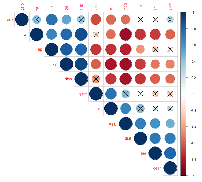
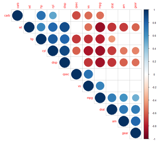
第 9 步：[添加显着性测试]：我们需要在corrplot()函数中添加sig.level 和 insig 参数。如果 p 值大于 0.01，则它是一个无关紧要的值，单元格要么是空白要么是交叉。

R

# Correlogram in R
# required package
library(corrplot)
  
head(mtcars)
M<-cor(mtcars)
head(round(M, 2))
  
library(corrplot)
  
# mat : is a matrix of data
# ... : further arguments to pass 
# to the native R cor.test function
cor.mtest <- function(mat, ...)
{
  mat <- as.matrix(mat)
  n <- ncol(mat)
  p.mat<- matrix(NA, n, n)
  diag(p.mat) <- 0
  for (i in 1:(n - 1)) 
  {
    for (j in (i + 1):n)
    {
      tmp <- cor.test(mat[, i], mat[, j], ...)
      p.mat[i, j] <- p.mat[j, i] <- tmp$p.value
    }
  }
  colnames(p.mat) <- rownames(p.mat) <- colnames(mat)
  p.mat
}
  
# matrix of the p-value of the correlation
p.mat <- cor.mtest(mtcars)
head(p.mat[, 1:5])
  
# Specialized the insignificant value
# according to the significant level
corrplot(M, type = "upper", order = "hclust", 
         p.mat = p.mat, sig.level = 0.01)
  
# Leave blank on no significant coefficient
corrplot(M, type = "upper", order = "hclust", 
         p.mat = p.mat, sig.level = 0.01, 
         insig = "blank")

输出：

第 10 步：[自定义相关图]：我们可以使用corrplot()函数中所需的参数并调整它们的值来自定义我们的相关图。

R

# Correlogram in R
# required package
library(corrplot)
library(RColorBrewer)
  
head(mtcars)
M<-cor(mtcars)
head(round(M,2))
  
# customize the correlogram
library(corrplot)
col <- colorRampPalette(c("#BB4444", "#EE9988", 
                          "#FFFFFF", "#77AADD",
                          "#4477AA"))
  
corrplot(M, method = "color", col = col(200),  
         type = "upper", order = "hclust", 
         addCoef.col = "black", # Add coefficient of correlation
         tl.col="black", tl.srt = 45, # Text label color and rotation
           
         # Combine with significance
         p.mat = p.mat, sig.level = 0.01, insig = "blank", 
           
         # hide correlation coefficient
         # on the principal diagonal
         diag = FALSE 
)

输出：