R 编程中的描述性分析

在描述性分析中，我们借助各种具有代表性的方法来描述我们的数据，例如使用图表、图形、表格、Excel 文件等。在描述性分析中，我们以某种方式描述我们的数据并以有意义的方式呈现它，以便很容易理解。大多数情况下，它是在小数据集上执行的，这种分析有助于我们根据当前的发现预测一些未来的趋势。用于描述数据集的一些度量是集中趋势的度量和可变性或离散度的度量。

描述性分析过程

• 集中趋势的度量
• 可变性的测量

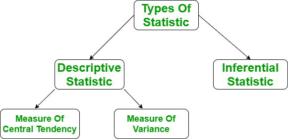
集中趋势的度量

它用单个值表示整个数据集。它为我们提供了中心点的位置。集中趋势的三个主要指标：

• 意思是
• 模式
• 中位数

可变性的测量

可变性的度量被称为数据的传播或我们的数据分布的好坏。最常见的可变性测量是：

• 范围
• 方差
• 标准差

需要描述性分析

描述性分析帮助我们理解我们的数据，是机器学习中非常重要的一部分。这是因为机器学习都是关于做出预测的。另一方面，统计学就是从数据中得出结论，这是机器学习的必要初始步骤。让我们在 R 中进行描述性分析。

R中的描述性分析

描述性分析包括使用一些汇总统计数据和图形简单地描述数据。在这里，我们将描述如何使用 R 软件计算汇总统计数据。

将数据导入 R：

在进行任何计算之前，首先，我们需要准备数据，将数据保存在外部 .txt 或 .csv 文件中，最好将文件保存在当前目录中。导入后，您的数据到 R 中，如下所示：

在此处获取 csv 文件。

R

# R program to illustrate
# Descriptive Analysis
 
# Import the data using read.csv()
myData = read.csv("CardioGoodFitness.csv",
                stringsAsFactors = F)
# Print the first 6 rows
print(head(myData))

输出：

Product Age Gender Education MaritalStatus Usage Fitness Income Miles
1   TM195  18   Male        14        Single     3       4  29562   112
2   TM195  19   Male        15        Single     2       3  31836    75
3   TM195  19 Female        14     Partnered     4       3  30699    66
4   TM195  19   Male        12        Single     3       3  32973    85
5   TM195  20   Male        13     Partnered     4       2  35247    47
6   TM195  20 Female        14     Partnered     3       3  32973    66

用于计算描述性分析的 R 函数：

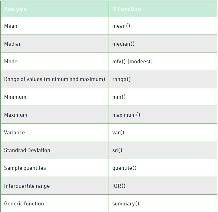
意思是

它是观测值的总和除以观测值的总数。它也被定义为平均值，即总和除以计数。

其中 n = 项数

例子：

R

# R program to illustrate
# Descriptive Analysis
 
# Import the data using read.csv()
myData = read.csv("CardioGoodFitness.csv",
                stringsAsFactors = F)
 
# Compute the mean value
mean = mean(myData$Age)
print(mean)

输出：

[1] 28.78889

中位数

它是数据集的中间值。它将数据分成两半。如果数据集中元素的数量是奇数，则中心元素是中值，如果是偶数，则中值将是两个中心元素的平均值。

其中 n = 项数

例子：

R

# R program to illustrate
# Descriptive Analysis
 
# Import the data using read.csv()
myData = read.csv("CardioGoodFitness.csv",
                stringsAsFactors = F)
 
# Compute the median value
median = median(myData$Age)
print(median)

输出：

[1] 26

模式

它是给定数据集中频率最高的值。如果所有数据点的频率相同，则数据集可能没有众数。此外，如果我们遇到两个或多个具有相同频率的数据点，我们可以有多个模式。

例子：

R

# R program to illustrate
# Descriptive Analysis
 
# Import the library
library(modeest)
 
# Import the data using read.csv()
myData = read.csv("CardioGoodFitness.csv",
                stringsAsFactors = F)
 
# Compute the mode value
mode = mfv(myData$Age)
print(mode)

输出：

[1] 25

范围

该范围描述了我们数据集中最大和最小数据点之间的差异。范围越大，数据的传播越多，反之亦然。

Range = Largest data value – smallest data value 

例子：

R

# R program to illustrate
# Descriptive Analysis
 
# Import the data using read.csv()
myData = read.csv("CardioGoodFitness.csv",
                stringsAsFactors = F)
 
# Calculate the maximum
max = max(myData$Age)
# Calculate the minimum
min = min(myData$Age)
# Calculate the range
range = max - min
 
cat("Range is:\n")
print(range)
 
# Alternate method to get min and max
r = range(myData$Age)
print(r)

输出：

Range is:
[1] 32

[1] 18 50

方差

它被定义为与平均值的平均平方偏差。它的计算方法是找出每个数据点与平均值之间的差异（也称为平均值），将它们平方，将它们全部相加，然后除以我们数据集中存在的数据点的数量。

在哪里，
N = 项数
u = 平均值

例子：

R

# R program to illustrate
# Descriptive Analysis
 
# Import the data using read.csv()
myData = read.csv("CardioGoodFitness.csv",
                stringsAsFactors = F)
 
# Calculating variance
variance = var(myData$Age)
print(variance)

输出：

[1] 48.21217

标准差

它被定义为方差的平方根。它是通过找到平均值来计算的，然后从平均值中减去每个数字，这也称为平均值，然后对结果进行平方。将所有值相加，然后除以平方根后的项数。

在哪里，
N = 项数
u = 平均值

例子：

R

# R program to illustrate
# Descriptive Analysis
 
# Import the data using read.csv()
myData = read.csv("CardioGoodFitness.csv", stringsAsFactors = F)
 
# Calculating Standard deviation
std = sd(myData$Age)
print(std)

输出：

[1] 6.943498

描述性分析中使用的更多 R函数：

四分位数

四分位数是一种分位数。第一个四分位数 (Q1) 定义为最小数字和数据集中位数之间的中间数，第二个四分位数 (Q2) – 给定数据集的中位数，而第三个四分位数 (Q3) 是中间数数据集的中位数和最大值之间的数字。

例子：

R

# R program to illustrate
# Descriptive Analysis
 
# Import the data using read.csv()
myData = read.csv("CardioGoodFitness.csv", stringsAsFactors = F)
 
# Calculating Quartiles
quartiles = quantile(myData$Age)
print(quartiles)

输出：

0%  25%  50%  75% 100% 
18   24   26   33   50 

四分位距

四分位间距 (IQR)，也称为中间价差或中间 50%，或技术上的 H 价差是第三四分位数 (Q3) 和第一四分位数 (Q1) 之间的差异。它覆盖了分布的中心并包含 50% 的观测值。

IQR = Q3 – Q1

例子：

R

# R program to illustrate
# Descriptive Analysis
 
# Import the data using read.csv()
myData = read.csv("CardioGoodFitness.csv", stringsAsFactors = F)
 
# Calculating IQR
IQR = IQR(myData$Age)
print(IQR)

输出：

[1] 9

R中的summary()函数

函数summary()可用于显示一个变量或整个数据框的多个统计摘要。

单个变量的摘要：

例子：

R

# R program to illustrate
# Descriptive Analysis
 
# Import the data using read.csv()
myData = read.csv("CardioGoodFitness.csv",
                stringsAsFactors = F)
 
# Calculating summary
summary = summary(myData$Age)
print(summary)

输出：

Min. 1st Qu.  Median    Mean 3rd Qu.    Max. 
18.00   24.00   26.00   28.79   33.00   50.00 

数据框摘要

例子：

R

# R program to illustrate
# Descriptive Analysis
 
# Import the data using read.csv()
myData = read.csv("CardioGoodFitness.csv",
                stringsAsFactors = F)
 
# Calculating summary
summary = summary(myData)
print(summary)

输出：

Product               Age           Gender            Education    
 Length:180         Min.   :18.00   Length:180         Min.   :12.00  
 Class :character   1st Qu.:24.00   Class :character   1st Qu.:14.00  
 Mode  :character   Median :26.00   Mode  :character   Median :16.00  
                    Mean   :28.79                      Mean   :15.57  
                    3rd Qu.:33.00                      3rd Qu.:16.00  
                    Max.   :50.00                      Max.   :21.00  


 MaritalStatus          Usage          Fitness          Income           Miles      
 Length:180         Min.   :2.000   Min.   :1.000   Min.   : 29562   Min.   : 21.0  
 Class :character   1st Qu.:3.000   1st Qu.:3.000   1st Qu.: 44059   1st Qu.: 66.0  
 Mode  :character   Median :3.000   Median :3.000   Median : 50597   Median : 94.0  
                    Mean   :3.456   Mean   :3.311   Mean   : 53720   Mean   :103.2  
                    3rd Qu.:4.000   3rd Qu.:4.000   3rd Qu.: 58668   3rd Qu.:114.8  
                    Max.   :7.000   Max.   :5.000   Max.   :104581   Max.   :360.0