Python中的图形绘图 |设置 2

Python中的图形绘图 |设置 1

子图

当我们想在同一个图中显示两个或多个图时，需要子图。我们可以使用两种略有不同的方法以两种方式进行。
方法一

Python

# importing required modules
import matplotlib.pyplot as plt
import numpy as np
 
# function to generate coordinates
def create_plot(ptype):
    # setting the x-axis values
    x = np.arange(-10, 10, 0.01)
     
    # setting the y-axis values
    if ptype == 'linear':
        y = x
    elif ptype == 'quadratic':
        y = x**2
    elif ptype == 'cubic':
        y = x**3
    elif ptype == 'quartic':
        y = x**4
             
    return(x, y)
 
# setting a style to use
plt.style.use('fivethirtyeight')
 
# create a figure
fig = plt.figure()
 
# define subplots and their positions in figure
plt1 = fig.add_subplot(221)
plt2 = fig.add_subplot(222)
plt3 = fig.add_subplot(223)
plt4 = fig.add_subplot(224)
 
# plotting points on each subplot
x, y = create_plot('linear')
plt1.plot(x, y, color ='r')
plt1.set_title('$y_1 = x$')
 
x, y = create_plot('quadratic')
plt2.plot(x, y, color ='b')
plt2.set_title('$y_2 = x^2$')
 
x, y = create_plot('cubic')
plt3.plot(x, y, color ='g')
plt3.set_title('$y_3 = x^3$')
 
x, y = create_plot('quartic')
plt4.plot(x, y, color ='k')
plt4.set_title('$y_4 = x^4$')
 
# adjusting space between subplots
fig.subplots_adjust(hspace=.5,wspace=0.5)
 
# function to show the plot
plt.show()

输出：

让我们逐步完成这个程序：

plt.style.use('fivethirtyeight')

• 可以通过设置不同的可用样式或设置您自己的样式来配置绘图的样式。您可以在此处了解有关此功能的更多信息

fig = plt.figure()

• Figure 充当所有绘图元素的顶级容器。因此，我们将一个图形定义为fig ，它将包含我们所有的子图。

plt1 = fig.add_subplot(221)
plt2 = fig.add_subplot(222)
plt3 = fig.add_subplot(223)
plt4 = fig.add_subplot(224)

• 这里我们使用 fig.add_subplot 方法来定义子图及其位置。函数原型是这样的：

add_subplot(nrows, ncols, plot_number)

• 如果将子图应用于图形，则图形理论上将被拆分为“nrows”*“ncols”子轴。参数“plot_number”标识函数调用必须创建的子图。 'plot_number' 的范围可以从 1 到最大 'nrows' * 'ncols'。
  如果三个参数的值小于 10，则可以使用一个 int 参数调用函数subplot，其中百位代表“nrows”，十位代表“ncols”，个位代表“plot_number”。这意味着：我们可以写subplot(234)而不是subplot(2, 3, 4 ) 。
  该图将清楚地表明如何指定位置：

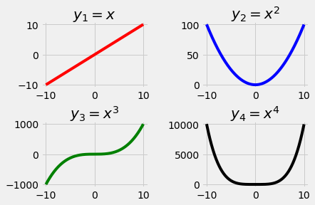
x, y = create_plot('linear')
plt1.plot(x, y, color ='r')
plt1.set_title('$y_1 = x$')

• 接下来，我们在每个子图上绘制我们的点。首先，我们使用create_plot函数通过指定我们想要的曲线类型来生成 x 和 y 轴坐标。
  然后，我们使用.plot方法在子图上绘制这些点。使用set_title方法设置子图的标题。在标题文本的开头和结尾使用$将确保 '_'（下划线）被读取为下标，而 '^' 被读取为上标。

fig.subplots_adjust(hspace=.5,wspace=0.5)

• 这是另一种在子图之间创建空间的实用方法。

plt.show()

• 最后，我们调用 plt.show() 方法来显示当前图形。

方法二

Python

# importing required modules
import matplotlib.pyplot as plt
import numpy as np
 
# function to generate coordinates
def create_plot(ptype):
    # setting the x-axis values
    x = np.arange(0, 5, 0.01)
     
    # setting y-axis values
    if ptype == 'sin':
        # a sine wave
        y = np.sin(2*np.pi*x)
    elif ptype == 'exp':
        # negative exponential function
        y = np.exp(-x)
    elif ptype == 'hybrid':
        # a damped sine wave
        y = (np.sin(2*np.pi*x))*(np.exp(-x))
             
    return(x, y)
 
# setting a style to use
plt.style.use('ggplot')
 
# defining subplots and their positions
plt1 = plt.subplot2grid((11,1), (0,0), rowspan = 3, colspan = 1)
plt2 = plt.subplot2grid((11,1), (4,0), rowspan = 3, colspan = 1)
plt3 = plt.subplot2grid((11,1), (8,0), rowspan = 3, colspan = 1)
 
# plotting points on each subplot
x, y = create_plot('sin')
plt1.plot(x, y, label = 'sine wave', color ='b')
x, y = create_plot('exp')
plt2.plot(x, y, label = 'negative exponential', color = 'r')
x, y = create_plot('hybrid')
plt3.plot(x, y, label = 'damped sine wave', color = 'g')
 
# show legends of each subplot
plt1.legend()
plt2.legend()
plt3.legend()
 
# function to show plot
plt.show()

输出：

让我们来看看这个程序的重要部分：

plt1 = plt.subplot2grid((11,1), (0,0), rowspan = 3, colspan = 1)
plt2 = plt.subplot2grid((11,1), (4,0), rowspan = 3, colspan = 1)
plt3 = plt.subplot2grid((11,1), (8,0), rowspan = 3, colspan = 1)

• subplot2grid类似于“pyplot.subplot”，但使用基于 0 的索引并让 subplot 占据多个单元格。
  让我们试着理解subplot2grid方法的参数：
  1. 论点 1：网格的几何形状
  2.参数2：网格中子图的位置
  3.参数3：（rowspan）子图覆盖的行数。
  4.参数4：（colspan）子图覆盖的列数。
  这张图会让这个概念更加清晰：

• 在我们的示例中，每个子图跨越 3 行和 1 列，其中包含两个空行（第 4,8 行）。

x, y = create_plot('sin')
plt1.plot(x, y, label = 'sine wave', color ='b')

• 这部分没有什么特别之处，因为在子图上绘制点的语法保持不变。

plt1.legend()

• 这将在图中显示子图的标签。

plt.show()

• 最后，我们调用 plt.show()函数来显示当前绘图。

注意：通过上述两个示例后，我们可以推断当图的大小一致时应该使用subplot()方法，而当我们希望子图的位置和大小具有更大的灵活性时，应该首选 subplot2grid() 方法。

3-D 绘图

我们可以在 matplotlib 中轻松绘制 3-D 图形。现在，我们讨论一些重要且常用的 3-D 图。

• 绘图点

Python

from mpl_toolkits.mplot3d import axes3d
import matplotlib.pyplot as plt
from matplotlib import style
import numpy as np
 
# setting a custom style to use
style.use('ggplot')
 
# create a new figure for plotting
fig = plt.figure()
 
# create a new subplot on our figure
# and set projection as 3d
ax1 = fig.add_subplot(111, projection='3d')
 
# defining x, y, z co-ordinates
x = np.random.randint(0, 10, size = 20)
y = np.random.randint(0, 10, size = 20)
z = np.random.randint(0, 10, size = 20)
 
# plotting the points on subplot
 
 
# setting labels for the axes
ax1.set_xlabel('x-axis')
ax1.set_ylabel('y-axis')
ax1.set_zlabel('z-axis')
 
# function to show the plot
plt.show()

• 上述程序的输出将为您提供一个可以旋转或放大绘图的窗口。这是一个屏幕截图：（暗点比亮点更近）

• 现在让我们试着理解这段代码的一些重要方面。

from mpl_toolkits.mplot3d import axes3d

• 这是在 3-D 空间上绘图所需的模块。

ax1 = fig.add_subplot(111, projection='3d')

• 在这里，我们在图形上创建一个子图并将投影参数设置为 3d。

ax1.scatter(x, y, z, c = 'm', marker = 'o')

• 现在我们使用.scatter()函数在 XYZ 平面上绘制点。
• 绘图线

Python

# importing required modules
from mpl_toolkits.mplot3d import axes3d
import matplotlib.pyplot as plt
from matplotlib import style
import numpy as np
 
# setting a custom style to use
style.use('ggplot')
 
# create a new figure for plotting
fig = plt.figure()
 
# create a new subplot on our figure
ax1 = fig.add_subplot(111, projection='3d')
 
# defining x, y, z co-ordinates
x = np.random.randint(0, 10, size = 5)
y = np.random.randint(0, 10, size = 5)
z = np.random.randint(0, 10, size = 5)
 
# plotting the points on subplot
ax1.plot_wireframe(x,y,z)
 
# setting the labels
ax1.set_xlabel('x-axis')
ax1.set_ylabel('y-axis')
ax1.set_zlabel('z-axis')
 
plt.show()

• 上述程序的 3-D 图的屏幕截图如下所示：

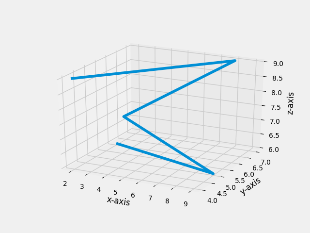
• 该程序与上一个程序的主要区别是：

ax1.plot_wireframe(x,y,z)

• 我们使用.plot_wireframe()方法在一组给定的 3-D 点上绘制线。
• 绘图条

Python

# importing required modules
from mpl_toolkits.mplot3d import axes3d
import matplotlib.pyplot as plt
from matplotlib import style
import numpy as np
 
# setting a custom style to use
style.use('ggplot')
 
# create a new figure for plotting
fig = plt.figure()
 
# create a new subplot on our figure
ax1 = fig.add_subplot(111, projection='3d')
 
# defining x, y, z co-ordinates for bar position
x = [1,2,3,4,5,6,7,8,9,10]
y = [4,3,1,6,5,3,7,5,3,7]
z = np.zeros(10)
 
# size of bars
dx = np.ones(10)              # length along x-axis
dy = np.ones(10)              # length along y-axs
dz = [1,3,4,2,6,7,5,5,10,9]   # height of bar
 
# setting color scheme
color = []
for h in dz:
    if h > 5:
        color.append('r')
    else:
        color.append('b')
 
# plotting the bars
ax1.bar3d(x, y, z, dx, dy, dz, color = color)
 
# setting axes labels
ax1.set_xlabel('x-axis')
ax1.set_ylabel('y-axis')
ax1.set_zlabel('z-axis')
 
plt.show()

• 创建的 3-D 环境的屏幕截图如下：

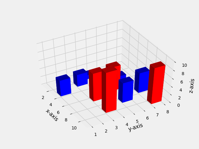
• 让我们来看看这个程序的重要方面：

x = [1,2,3,4,5,6,7,8,9,10]
y = [4,3,1,6,5,3,7,5,3,7]
z = np.zeros(10)

• 在这里，我们定义柱的基本位置。设置 z = 0 表示所有条形都从 XY 平面开始。

dx = np.ones(10)              # length along x-axis
dy = np.ones(10)              # length along y-axs
dz = [1,3,4,2,6,7,5,5,10,9]   # height of bar

• dx, dy, dz 表示条的大小。把他的 bar 看成一个长方体，那么 dx, dy, dz 分别是它沿 x, y, z 轴的展开。

for h in dz:
    if h > 5:
        color.append('r')
    else:
        color.append('b')

• 在这里，我们将每个条形的颜色设置为一个列表。高度大于 5 的条的配色方案为红色，否则为蓝色。

ax1.bar3d(x, y, z, dx, dy, dz, color = color)

• 最后，为了绘制条形图，我们使用.bar3d()函数。
• 绘制曲线

Python

# importing required modules
from mpl_toolkits.mplot3d import axes3d
import matplotlib.pyplot as plt
from matplotlib import style
import numpy as np
 
# setting a custom style to use
style.use('ggplot')
 
# create a new figure for plotting
fig = plt.figure()
 
# create a new subplot on our figure
ax1 = fig.add_subplot(111, projection='3d')
 
# get points for a mesh grid
u, v = np.mgrid[0:2*np.pi:200j, 0:np.pi:100j]
 
# setting x, y, z co-ordinates
x=np.cos(u)*np.sin(v)
y=np.sin(u)*np.sin(v)
z=np.cos(v)
 
# plotting the curve
ax1.plot_wireframe(x, y, z, rstride = 5, cstride = 5, linewidth = 1)
 
plt.show()

• 该程序的输出将如下所示：
  

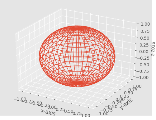
• 在这里，我们将球体绘制为网格。
  让我们来看看一些重要的部分：

u, v = np.mgrid[0:2*np.pi:200j, 0:np.pi:100j]

• 我们使用 np.mgrid 来获取点，以便我们可以创建网格。
  您可以在此处阅读有关此内容的更多信息。

x=np.cos(u)*np.sin(v)
y=np.sin(u)*np.sin(v)
z=np.cos(v)

• 这不过是球体的参数方程。

ax1.plot_wireframe(x, y, z, rstride = 5, cstride = 5, linewidth = 1)

• Agan，我们使用.plot_wireframe()方法。在这里，可以使用rstride和cstride参数来设置我们的网格必须有多大的密度。