在 R 中划分 ggplot2 图的图例

在本文中，我们将讨论如何在 R 编程语言中划分 ggplot2 图的图例。

要划分ggplot2图的图例，用户需要在R控制台中安装并导入gridExtra和cowplot包。

• gridExrta 包：提供许多用户级函数来处理“网格”图形，特别是在页面上排列多个基于网格的图，并绘制表格。
• cowplot 包： cowplot 包是 ggplot 的一个简单附加组件。它提供了有助于创建出版质量图形的各种功能，例如一组主题、对齐绘图并将它们排列成复杂复合图形的函数，以及使注释绘图和/或将绘图与图像混合的功能。

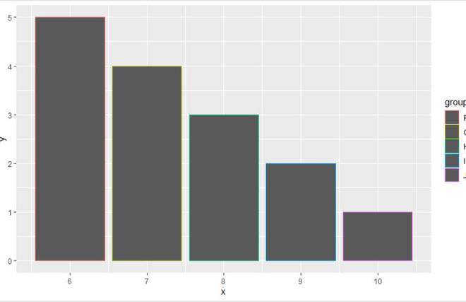
让我们先创建一个包含所有图例的情节，然后再将它们分开，以便差异更加明显。

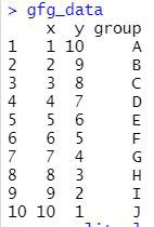
使用中的数据：

例子：

R

library(ggplot2)
library(gridExtra)
library(cowplot)
  
gfg_data <- data.frame(x = 1:10, y = 10:1, group = LETTERS[1:10])
  
ggp_plot<- ggplot(gfg_data, aes(x,y,color = group)) + 
geom_bar(stat="identity") +scale_color_manual(values = 1:10) +
labs(color = "Legend-1")
  
ggp_plot

输出：

要划分图例，请从数据框中提取较小的数据样本，并应用具有适当参数的所需函数来生成所需的图。

例子：

电阻

# legends for two
library(ggplot2)
library(gridExtra)
library(cowplot)
  
gfg_data <- data.frame(x = 1:10, y = 10:1, group = LETTERS[1:10])
  
gfg_split_1 <- gfg_data[gfg_data$group %in% c("A", "B"), ]   
gfg_split_1
  
ggp_split_plot_1 <- ggplot(gfg_split_1, aes(x,y,color = group)) + 
geom_bar(stat="identity")+scale_color_manual(values = 1:2) +
labs(color = "Legend-1")
ggp_split_plot_1  

输出：

例子：

电阻

# legends for three
library(ggplot2)
library(gridExtra)
library(cowplot)
  
gfg_data <- data.frame(x = 1:10, y = 10:1, group = LETTERS[1:10])
  
gfg_split_2 <- gfg_data[gfg_data$group %in% c("C", "D","E"), ] 
gfg_split_2
  
ggp_split_plot_2 <- ggplot(gfg_split_2, aes(x,y,color = group)) + 
geom_bar(stat="identity")+
scale_color_manual(values = 1:3) +labs(color = "Legend-1")
  
ggp_split_plot_2  

输出：

例子：

电阻

# legends for rest of the data
library(ggplot2)
library(gridExtra)
library(cowplot)
  
gfg_data <- data.frame(x = 1:10, y = 10:1, group = LETTERS[1:10])
  
gfg_split_3 <- gfg_data[! gfg_data$group %in% c("A","B","C", "D","E"), ]
gfg_split_3
  
ggp_split_plot_3 <- ggplot(gfg_split_3, aes(x,y,color = group)) + 
geom_bar(stat="identity")+scale_color_manual(values = 1:5) + 
labs(color = "Legend-1")
  
ggp_split_plot_3  

输出：