霍普菲尔德神经网络

先决条件： RNN

由 John J. Hopfield 博士发明的 Hopfield 神经网络由一层“n”个完全连接的循环神经元组成。它通常用于执行自动关联和优化任务。它是使用收敛的交互过程计算的，它产生与我们普通神经网络不同的响应。

离散 Hopfield 网络：它是一个完全互连的神经网络，其中每个单元都连接到其他每个单元。它以离散方式运行，即它提供有限的不同输出，通常有两种类型：

• 二进制 (0/1)
• 双极 (-1/1)

与该网络相关的权重本质上是对称的，并具有以下特性。

$1.\ w_{ij} = w_{ji} \\ 2.\ w_{ii} = 0$

结构与架构

• 每个神经元都有一个反相和一个非反相输出。
• 在完全连接的情况下，每个神经元的输出是所有其他神经元的输入，而不是自身。

图 1显示了具有以下元素的离散 Hopfield 神经网络架构的示例表示。

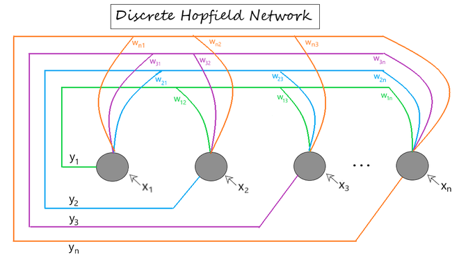
图 1：离散 Hopfield 网络架构

[ x1 , x2 , ... , xn ] -> Input to the n given neurons.
[ y1 , y2 , ... , yn ] -> Output obtained from the n given neurons
Wij -> weight associated with the connection between the ith and the jth neuron.

训练算法

为了存储一组输入模式 S(p) [p = 1 到 P]，其中S(p) = S ₁ (p) … S _i (p) … S _n (p) ，权重矩阵由下式给出：

• 对于二进制模式

$w_{ij} = \sum_{p = 1}^{P} [2s_{i}(p) - 1][2s_{j}(p) - 1]\ (w_{ij}\ for\ all\ i\neq j)$

• 对于双极模式

$w_{ij} = \sum_{p = 1}^{P} [s_{i}(p)s_{j}(p)]\ (where\ w_{ij} = 0\ for\ all\ i= j)$

（即这里的权重没有自连接）

涉及步骤

Step 1 - Initialize weights (wij) to store patterns (using training algorithm).

Step 2 - For each input vector yi, perform steps 3-7.

Step 3 - Make initial activators of the network equal to the external input vector x. 

$y_i = x_i : (for\ i = 1\ to\ n)$

Step 4 - For each vector yi, perform steps 5-7. 

Step 5 - Calculate the total input of the network yin using the equation given below.

$y_{in_{i}} = x_i + \sum_{j} [y_jw_{ji}]$

Step 6 - Apply activation over the total input to calculate the output as per the equation given below: 

$y_i = \begin{cases} & 1 \text{ if } y_{in}>\theta_i \\ & y_i \text{ if } y_{in}=\theta_i \\ & 0 \text{ if } y_{in}<\theta_i \end{cases}$

（其中θ _i （阈值）通常取为 0）

Step 7 - Now feedback the obtained output yi to all other units. Thus, the activation vectors are updated.

Step 8 - Test the network for convergence.

示例问题

考虑以下问题。我们需要创建具有输入向量双极表示的离散 Hopfield 网络，因为 [1 1 1 -1] 或 [1 1 1 0]（在二进制表示的情况下）存储在网络中。使用存储向量的第一个和第二个分量（即 [0 0 1 0]）中缺失的条目测试 hopfield 网络。

分步解决方案

Step 1 - given input vector, x = [1 1 1 -1] (bipolar) and we initialize the weight matrix (wij) as:

$w_{ij} = \sum [s^T(p)t(p)] \\ = \begin{bmatrix} 1 \\ 1 \\ 1 \\ -1 \end{bmatrix} \begin{bmatrix} 1 & 1 & 1 & -1 \end{bmatrix} \\ = \begin{bmatrix} 1 & 1 & 1 & -1 \\ 1 & 1 & 1 & -1 \\ 1 & 1 & 1 & -1 \\ -1 & -1 & -1 & 1 \\\end{bmatrix}$

and weight matrix with no self connection is:

$w_{ij} = \begin{bmatrix} 0 & 1 & 1 & -1 \\ 1 & 0 & 1 & -1 \\ 1 & 1 & 0 & -1 \\ -1 & -1 & -1 & 0 \\\end{bmatrix}$

Step 3 - As per the question, input vector x with missing entries, x = [0 0 1 0] ([x1 x2 x3 x4]) (binary)
       - Make yi = x = [0 0 1 0] ([y1 y2 y3 y4])

Step 4 - Choosing unit yi (order doesn't matter) for updating its activation. 
       - Take the ith column of the weight matrix for calculation.        
 
(we will do the next steps for all values of yi and check if there is convergence or not) 

$y_{in_{1}} = x_1 + \sum_{j = 1}^4 [y_j w_{j1}] \\ = 0\ + \begin{bmatrix} 0 & 0 & 1 & 0 \end{bmatrix} \begin{bmatrix} 0 \\ 1 \\ 1 \\ -1 \end{bmatrix} \\ = 0\ + 1 \\ = 1 \\ Applying\ activation,\ y_{in_1} > 0 \implies y_1 = 1 \\ giving\ feedback\ to\ other\ units,\ we\ get \\ y = \begin{bmatrix} 1 & 0 & 1 & 0 \end{bmatrix} \\ which\ is\ not\ equal\ to\ input\ vector\ \\ x = \begin{bmatrix} 1 & 1 & 1 & 0 \end{bmatrix} \\ Hence,\ no\ covergence.$ '

now for next unit, we will take updated value via feedback. (i.e. y = [1 0 1 0]) 

$y_{in_{3}} = x_3 + \sum_{j = 1}^4 [y_j w_{j3}] \\ = 1\ + \begin{bmatrix} 1 & 0 & 1 & 0 \end{bmatrix} \begin{bmatrix} 1 \\ 1 \\ 0 \\ -1 \end{bmatrix} \\ = 1\ + 1 \\ = 2 \\ Applying\ activation,\ y_{in_3} > 0 \implies y_3= 1 \\ giving\ feedback\ to\ other\ units,\ we\ get \\ y = \begin{bmatrix} 1 & 0 & 1 & 0 \end{bmatrix} \\ which\ is\ not\ equal\ to\ input\ vector\ \\ x = \begin{bmatrix} 1 & 1 & 1 & 0 \end{bmatrix} \\ Hence,\ no\ covergence.$

now for next unit, we will take updated value via feedback. (i.e. y = [1 0 1 0])

$y_{in_{4}} = x_4 + \sum_{j = 1}^4 [y_j w_{j4}] \\ = 0\ + \begin{bmatrix} 1 & 0 & 1 & 0 \end{bmatrix} \begin{bmatrix} -1 \\ -1 \\ -1 \\ 0 \end{bmatrix} \\ = 0\ + (-1)\ + (-1) \\ = -2 \\ Applying\ activation,\ y_{in_4} < 0 \implies y_4= 0 \\ giving\ feedback\ to\ other\ units,\ we\ get \\ y = \begin{bmatrix} 1 & 0 & 1 & 0 \end{bmatrix} \\ which\ is\ not\ equal\ to\ input\ vector\ \\ x = \begin{bmatrix} 1 & 1 & 1 & 0 \end{bmatrix} \\ Hence,\ no\ covergence.$

now for next unit, we will take updated value via feedback. (i.e. y = [1 0 1 0])

$y_{in_{2}} = x_2 + \sum_{j = 1}^4 [y_j w_{j2}] \\ = 0\ + \begin{bmatrix} 1 & 0 & 1 & 0 \end{bmatrix} \begin{bmatrix} 1 \\ 0 \\ 1 \\ -1 \end{bmatrix} \\ = 0\ + 1\ + 1 \\ = 2 \\ Applying\ activation,\ y_{in_2} > 0 \implies y_2= 1 \\ giving\ feedback\ to\ other\ units,\ we\ get \\ y = \begin{bmatrix} 1 & 1 & 1 & 0 \end{bmatrix} \\ which\ is\ equal\ to\ input\ vector\ \\ x = \begin{bmatrix} 1 & 1 & 1 & 0 \end{bmatrix} \\ Hence,\ covergence\ with\ vector\ x.$

连续跳场网络：与离散跳场网络不同，这里的时间参数被视为连续变量。因此，我们可以获得介于 0 和 1 之间的值，而不是获得二进制/双极输出。它可用于解决约束优化和关联内存问题。输出定义为：

$v_i = g(u_i)$

where,
vi = output from the continuous hopfield network
ui = internal activity of a node in continuous hopfield network.

能量函数

跳场网络具有与之相关的能量函数。每次迭代后，它在更新（反馈）时要么减少要么保持不变。连续跳场网络的能量函数定义为：

$E = 0.5 \sum_{i=1}^n \sum_{j=1}^n w_{ij}v_i v_j + \sum_{i=1}^n \theta_i v_i$

为了确定网络是否会收敛到稳定配置，我们通过以下方式查看能量函数达到最小值：

$\frac{d}{dt} E \leq 0$

如果每个神经元的活动时间由以下微分方程给出，则网络一定会收敛：

$\frac{d}{dt}u_i = \frac{-u_i}{\tau} + \sum_{j=1}^n w_{ij} v_j + \theta_i$