从Web或其他资源下载的数据通常很难分析。通常需要对数据集进行一些处理或清理,以便为进一步的下游分析,预测建模等做准备。本文讨论了R中将原始数据集转换为整齐数据的几种方法。
原始数据
原始数据是已从Web(或任何其他来源)下载且尚未处理的数据集。原始数据尚未准备好用于统计。它需要各种处理工具才能进行分析。
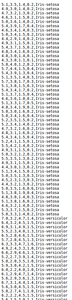
示例:下面是原始IRIS数据集的图像。它没有任何信息,如数据是什么或代表什么。这将通过整理数据来完成。
整理数据
另一方面,Tidy数据集(也称为熟数据)是具有以下特征的数据:
- 所测量的每个变量都应放在一栏中。
- 该变量的每个不同观察值都应位于不同的行中。
- 每种“种类”的变量都应该有一个表。
- 如果有多个表,则它们应该在表中包括一列,以允许将它们链接起来。
示例:以下是Tidy IRIS数据集的图像。它包含有价值的已处理信息,例如列名。该过程将在下面解释。

使用示例将原始数据集一般处理为整洁数据集的步骤
- 在R中加载数据集
- 第一步是获取要处理的数据。这里获取的数据来自IRIS数据。
- 首先下载数据并将其放入R中的数据框。
##Provide the link of the dataset
url < -"http:// archive.ics.uci.edu/ml/machine-learning-databases/iris/iris.data"

##download the data in a file iris.txt
##will be saved in the working directory
download.file(url, "iris.txt")

##import the data in a dataframe
d < -read.table("iris.txt", sep = ", ")

##Rename the columns
colnames(d)< -c("s_len",
         "s_width",
         "p_len",
         "p_width",
         "variety")
- 子集行和列
- 现在,如果仅需要s_len(第一列),p_len(第三列)和variant(第五列)进行分析,则将这些列作为子集,并将新数据分配给新数据框。
##subsetting columns with column number d1 <- d[, c(1, 3, 5)] - 子设置也可以使用列名来完成。
##subsetting columns with column names d1 <- d[, c("s_len", "p_len", "variety")] - 同样,如果需要知道“鸢尾花”变种或“树皮长度小于5”的观测值。
##Subsetting the rows
d2 <- d[(d$s_len < 5 | d$variety == "Iris-setosa"), ]
注意: “ $”运算符用于子集一列。
- 现在,如果仅需要s_len(第一列),p_len(第三列)和variant(第五列)进行分析,则将这些列作为子集,并将新数据分配给新数据框。
- 按某个变量对数据框进行排序
使用命令命令按花瓣长度对数据帧进行排序。
d3 < -d[order(d$p_len), ] - 添加新的行和列
通过cbind()添加新列,并通过rbind()添加新行。
##Extract the s_width column of d sepal_width <- d$s_width ##Add the column to d1 dataframe. d1 <- cbind(d1, sepal_width) - 概览数据概览
- 要获得已处理数据的概述,请在数据帧上调用summary()命令。
summary(d)输出“:
s_len s_width p_len p_width variety Min. :4.300 Min. :2.000 Min. :1.000 Min. :0.100 Iris-setosa :50 1st Qu.:5.100 1st Qu.:2.800 1st Qu.:1.600 1st Qu.:0.300 Iris-versicolor:50 Median :5.800 Median :3.000 Median :4.350 Median :1.300 Iris-virginica :50 Mean :5.843 Mean :3.054 Mean :3.759 Mean :1.199 3rd Qu.:6.400 3rd Qu.:3.300 3rd Qu.:5.100 3rd Qu.:1.800 Max. :7.900 Max. :4.400 Max. :6.900 Max. :2.500 - 获得概述,例如每个变量的类型,观察值的总数及其前几个值;使用str()命令。
str(d)输出:
'data.frame':    150 obs. of  5 variables:
 $ s_len  : num  5.1 4.9 4.7 4.6 5 5.4 4.6 5 4.4 4.9 ...
 $ s_width: num  3.5 3 3.2 3.1 3.6 3.9 3.4 3.4 2.9 3.1 ...
 $ p_len  : num  1.4 1.4 1.3 1.5 1.4 1.7 1.4 1.5 1.4 1.5 ...
 $ p_width: num  0.2 0.2 0.2 0.2 0.2 0.4 0.3 0.2 0.2 0.1 ...
 $ variety: Factor w/ 3 levels "Iris-setosa", ..: 1 1 1 1 1 1 1 1 1 1 ...
- 要获得已处理数据的概述,请在数据帧上调用summary()命令。
使用Melt()和Cast()重塑数据
- 重新组织数据的另一种方法是使用熔化和铸造功能。它们以reshape2包装形式存在。
## Create A Dummy Dataset d<-data.frame( name=c("Arnab", "Arnab", "Soumik", "Mukul", "Soumik"), year=c(2011, 2014, 2011, 2015, 2014), height=c(5, 6, 4, 3, 5), Weight=c(90, 89, 76, 85, 84)) ## View the dataset d输出:
name year height Weight 1 Arnab 2011 5 90 2 Arnab 2014 6 89 3 Soumik 2011 4 76 4 Mukul 2015 3 85 5 Soumik 2014 5 84 - 融合这些数据意味着将某些变量称为id变量(其他变量将作为度量变量)。现在,如果将name和year用作id变量,并将height和weight用作度量变量,那么新数据集中将有4列-name ,year,variable和value 。对于每个名称和年份,都会有要测量的变量及其值。
## Getting the reshape library
install.packages("reshape2")
library(reshape2)

## Configure the id variables, name and year
melt(d, id=c("name", "year"))
输出:
name year variable value 1 Arnab 2011 height 5 2 Arnab 2014 height 6 3 Soumik 2011 height 4 4 Mukul 2015 height 3 5 Soumik 2014 height 5 6 Arnab 2011 Weight 90 7 Aranb 2014 Weight 89 8 Soumik 2011 Weight 76 9 Mukul 2015 Weight 85 10 Soumik 2014 Weight 84 - 现在可以通过cast()函数以紧凑的形式转换熔融数据集。计算每个人的平均身高和体重。
##Save the molten dataset
d1<-melt(d, id=c("name", "year"))

##Now cast the data
d2 <-cast(d1, name~variable, mean)

## View the data
d2
输出:
name height Weight
1  Arnab    5.5   89.5
2  Mukul    3.0   85.0
3 Soumik    4.5   80.0
注意:R中还有其他一些软件包,例如dplyr和tidyr ,它们提供用于准备整洁数据的功能。