R 编程中的回归及其类型

回归分析是一种统计工具，用于估计两个或多个变量之间的关系。总是有一个响应变量和一个或多个预测变量。回归分析被广泛用于对数据进行相应的拟合，并进一步预测数据以进行预测。它使用因/响应变量和自/预测变量帮助企业和组织了解其产品在市场中的行为。在本文中，让我们借助示例了解 R 编程中不同类型的回归。

R中的回归类型

R编程中广泛使用的回归主要有三种类型。他们是：

• 线性回归
• 多重回归
• 逻辑回归

线性回归

线性回归模型是三种回归类型中广泛使用的模型之一。在线性回归中，估计两个变量之间的关系，即一个响应变量和一个预测变量。线性回归在图上生成一条直线。数学上

$y = ax + b$

where, 

• x indicates predictor or independent variable
• y indicates response or dependent variable
• a and b are coefficients

R中的实现

在 R 编程中， lm()函数用于创建线性回归模型。

Syntax: lm(formula)
Parameter: 
formula: represents the formula on which data has to be fitted To know about more optional parameters, use below command in console: help(“lm”) 

示例：在此示例中，让我们在图表上绘制线性回归线，并使用身高预测基于体重。

R

# R program to illustrate
# Linear Regression
 
# Height vector
x <- c(153, 169, 140, 186, 128,
       136, 178, 163, 152, 133)
 
# Weight vector
y <- c(64, 81, 58, 91, 47, 57,
       75, 72, 62, 49)
 
# Create a linear regression model
model <- lm(y~x)
 
# Print regression model
print(model)
 
# Find the weight of a person
# With height 182
df <- data.frame(x = 182)
res <-  predict(model, df)
cat("\nPredicted value of a person
               with height = 182")
print(res)
 
# Output to be present as PNG file
png(file = "linearRegGFG.png")
 
# Plot
plot(x, y, main = "Height vs Weight
                 Regression model")
abline(lm(y~x))
 
# Save the file.
dev.off()

输出：

Call:
lm(formula = y ~ x)

Coefficients:
(Intercept)            x  
   -39.7137       0.6847

Predicted value of a person with height = 182
      1 
84.9098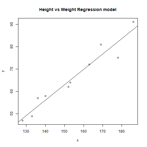

多重回归

多元回归是另一种类型的回归分析技术，它是线性回归模型的扩展，因为它使用多个预测变量来创建模型。数学上，

$y = a + x_1 * b_1 + x_2 * b_2 + ..... + x_n * b_n$

R中的实现

R 编程中的多元回归使用相同的lm()函数来创建模型。

Syntax: lm(formula, data)

Parameters:

• formula: represents the formula on which data has to be fitted
• data: represents dataframe on which formula has to be applied

示例：让我们创建 R 基础包中存在的空气质量数据集的多元回归模型，并将模型绘制在图表上。

R

# R program to illustrate
# Multiple Linear Regression
 
# Using airquality dataset
input <- airquality[1:50,
         c("Ozone", "Wind", "Temp")]
 
# Create regression model
model <- lm(Ozone~Wind + Temp,
            data = input)
 
# Print the regression model
cat("Regression model:\n")
print(model)
 
# Output to be present as PNG file
png(file = "multipleRegGFG.png")
 
# Plot
plot(model)
 
# Save the file.
dev.off()

输出：

Regression model:
Call:
lm(formula = Ozone ~ Wind + Temp, data = input)

Coefficients:
(Intercept)         Wind         Temp  
    -58.239       -0.739        1.329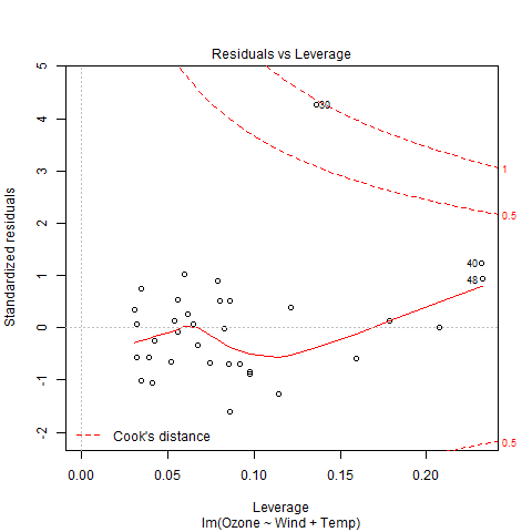

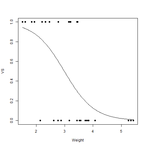
逻辑回归

Logistic Regression 是另一种广泛使用的回归分析技术，它用一个范围来预测值。此外，它用于预测分类数据的值。例如，电子邮件是垃圾邮件还是非垃圾邮件、赢家或输家、男性或女性等。从数学上讲，

$y=\frac{1}{1+e^{-z}}$

where, 

• y represents response variable
• z represents equation of independent variables or features

R中的实现

在 R 编程中， glm()函数用于创建逻辑回归模型。

Syntax: glm(formula, data, family)

Parameters: 

• formula: represents a formula on the basis of which model has to be fitted
• data: represents dataframe on which formula has to be applied
• family: represents the type of function to be used. “binomial” for logistic regression

例子：

R

# R program to illustrate
# Logistic Regression
 
# Using mtcars dataset
# To create the logistic model
model <- glm(formula = vs ~ wt,
             family = binomial,
             data = mtcars)
 
# Creating a range of wt values
x <- seq(min(mtcars$wt),
             max(mtcars$wt),
             0.01)
 
# Predict using weight
y <- predict(model, list(wt = x),
             type = "response")
 
# Print model
print(model)
 
# Output to be present as PNG file
png(file = "LogRegGFG.png")
 
# Plot
plot(mtcars$wt, mtcars$vs, pch = 16,
     xlab = "Weight", ylab = "VS")
lines(x, y)
 
# Saving the file
dev.off()

输出：

Call:  glm(formula = vs ~ wt, family = binomial, data = mtcars)

Coefficients:
(Intercept)           wt  
      5.715       -1.911  

Degrees of Freedom: 31 Total (i.e. Null);  30 Residual
Null Deviance:      43.86 
Residual Deviance: 31.37        AIC: 35.37