R 编程中的回归决策树

决策树是机器学习中的一种算法，它以决策为特征，以树状结构的形式表示结果。它是一种常用工具，用于直观地表示算法做出的决策。决策树同时使用分类和回归。当因变量是连续的时使用回归树，而当因变量是分类时使用分类树。例如，确定/预测性别是分类的示例，基于发动机功率预测汽车的里程是回归的示例。在本文中，让我们讨论 R 编程中使用回归的决策树以及 R 编程中的语法和实现。

R中的实现

在 R 编程中， rpart()函数存在于rpart包中。使用rpart()函数，可以在 R 中构建决策树。

Syntax:
rpart(formula, data, method)

Parameters:
formula: indicates the formula based on which model has to be fitted
data: indicates the dataframe
method: indicates the method to create decision tree. “anova” is used for regression and “class” is used as method for classification.

编程需要懂一点英语

示例 1：
在这个例子中，让我们使用回归决策树预测萼片宽度。

第一步：安装需要的包

# Install the package
install.packages("rpart")

第 2 步：加载包

# Load the package
library(rpart)

第 3 步：拟合回归决策树模型

# Create decision tree using regression
fit <- rpart(Sepal.Width ~ Sepal.Length + 
             Petal.Length + Petal.Width + Species, 
             method = "anova", data = iris)

第 4 步：绘制树

# Output to be present as PNG file
png(file = "decTreeGFG.png", width = 600, 
                            height = 600)
  
# Plot
plot(fit, uniform = TRUE,
          main = "Sepal Width Decision 
                 Tree using Regression")
text(fit, use.n = TRUE, cex = .7)
  
# Saving the file
dev.off()

第 5 步：打印决策树模型

# Print model
print(fit)

第 6 步：预测萼片宽度

# Create test data
df  <- data.frame (Species = 'versicolor', 
                   Sepal.Length = 5.1,
                   Petal.Length = 4.5,
                   Petal.Width = 1.4)
  
# Predicting sepal width
# using testing data and model
# method anova is used for regression
cat("Predicted value:\n")
predict(fit, df, method = "anova")

输出：

输出图

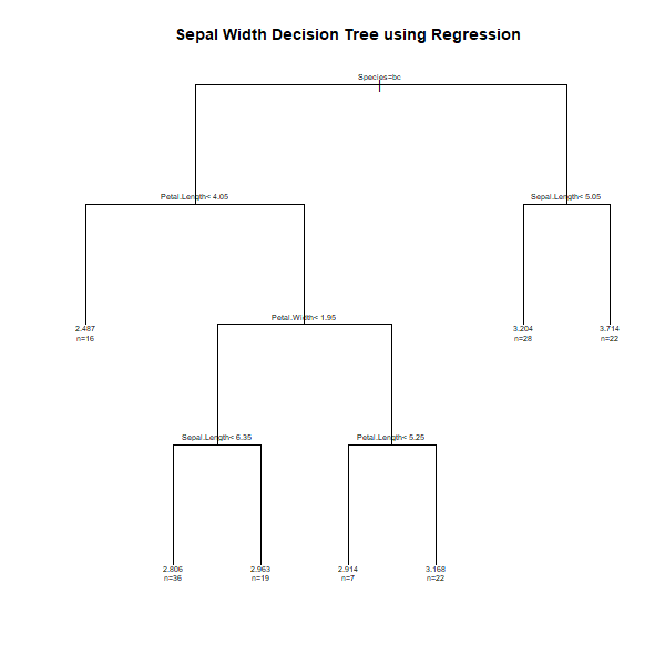
n= 150 

node), split, n, deviance, yval
      * denotes terminal node

 1) root 150 28.3069300 3.057333  
   2) Species=versicolor, virginica 100 10.9616000 2.872000  
     4) Petal.Length=4.05 84  7.3480950 2.945238  
      10) Petal.Width< 1.95 55  3.4920000 2.860000  
        20) Sepal.Length=6.35 19  0.6242105 2.963158 *
      11) Petal.Width>=1.95 29  2.6986210 3.106897  
        22) Petal.Length=5.25 22  2.0277270 3.168182 *
   3) Species=setosa 50  7.0408000 3.428000  
     6) Sepal.Length=5.05 22  1.7859090 3.713636 *

Predicted value:
       1 
2.805556

示例 2：
在此示例中，让我们使用决策树进行回归预测 mpg 值。

第一步：安装需要的包

# Install the package
install.packages("rpart")

第 2 步：加载包

# Load the package
library(rpart)

第 3 步：拟合回归决策树模型

# Create decision tree using regression
fit <- rpart(mpg ~ disp + hp + cyl, 
method = "anova", data = mtcars )

第 4 步：绘制树

# Output to be present as PNG file
png(file = "decTree2GFG.png", width = 600,
                             height = 600)
  
# Plot
plot(fit, uniform = TRUE,
main = "MPG Decision Tree using Regression")
text(fit, use.n = TRUE, cex = .6)
  
# Saving the file
dev.off()

第 5 步：打印决策树模型

# Print model
print(fit)

第 6 步：使用测试数据集预测 mpg 值

# Create test data
df  <- data.frame (disp = 351, hp = 250, 
                                cyl = 8)
  
# Predicting mpg using testing data and model
cat("Predicted value:\n")
predict(fit, df, method = "anova")

输出：

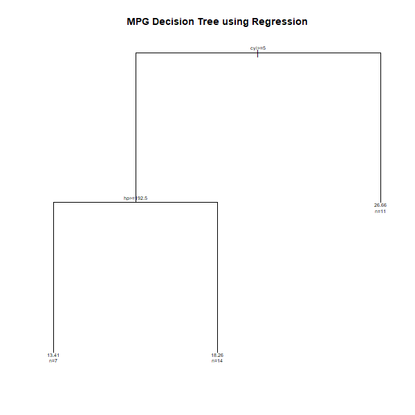
n= 32 

node), split, n, deviance, yval
      * denotes terminal node

1) root 32 1126.04700 20.09062  
  2) cyl>=5 21  198.47240 16.64762  
    4) hp>=192.5 7   28.82857 13.41429 *
    5) hp< 192.5 14   59.87214 18.26429 *
  3) cyl< 5 11  203.38550 26.66364 *

Predicted value:
       1 
13.41429

决策树的优势

考虑所有可能的决策：决策树考虑所有可能的决策以产生问题的结果。
易于使用：借助分类和回归技术，它可以轻松用于任何类型的问题，并进一步创建预测和解决问题。
缺失值没有问题：数据集缺失值没有问题，不影响决策树的构建。

决策树的缺点

需要更长的时间：决策树需要更长的时间来计算大型数据集。
学习少：决策树不是好的学习者。随机森林方法用于更好的学习。