Matplotlib 3D 绘图简介

在本文中，我们将学习使用Matplotlib 进行3D 绘图。我们可以通过多种方式使用 matplotlib 创建 3D 绘图，例如创建一个空画布并向其添加轴，您将投影定义为 3D 投影Matplotlib.pyplot.gca() ， 等等。

创建一个空的 3D 绘图：

在下面的代码中，我们将首先创建一个空画布。之后，我们将定义 3D 绘图的轴，其中我们定义绘图的投影将采用“ 3D ”格式。这有助于我们在画布中创建 3D 空轴图形。在此之后，如果我们使用plt.show()显示绘图，那么它看起来就像输出中显示的那样。

示例：使用 Matplotlib 创建一个空的 3D 图

Python3

# importing numpy package from
# python library
import numpy as np
 
# importing matplotlib.pyplot package from
# python
import matplotlib.pyplot as plt
 
# Creating an empty figure
# or plot
fig = plt.figure()
 
# Defining the axes as a
# 3D axes so that we can plot 3D
# data into it.
ax = plt.axes(projection="3d")
 
# Showing the above plot
plt.show()

输出：

现在，我们对如何在空画布上创建 3D 绘图有了基本的了解。让我们转到一些 3D 绘图示例。

3D 绘图示例：

示例 1：

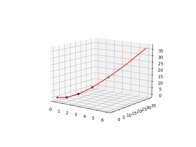
在下面的示例中，我们将在 3D 图中绘制一条简单的曲线。与此同时，我们将绘制一系列具有 X 坐标、Y 坐标和 Z 坐标的点。

蟒蛇3

# importing numpy package
import numpy as np
 
# importing matplotlib package
import matplotlib.pyplot as plt
 
# importing mplot3d from
# mpl_toolkits
from mpl_toolkits import mplot3d
 
# creating an empty canvas
fig = plt.figure()
 
# defining the axes with the projection
# as 3D so as to plot 3D graphs
ax = plt.axes(projection="3d")
 
# creating a wide range of points x,y,z
x=[0,1,2,3,4,5,6]
y=[0,1,4,9,16,25,36]
z=[0,1,4,9,16,25,36]
 
# plotting a 3D line graph with X-coordinate,
# Y-coordinate and Z-coordinate respectively
ax.plot3D(x, y, z, 'red')
 
# plotting a scatter plot with X-coordinate,
# Y-coordinate and Z-coordinate respectively
# and defining the points color as cividis
# and defining c as z which basically is a
# defination of 2D array in which rows are RGB
#or RGBA
ax.scatter3D(x, y, z, c=z, cmap='cividis');
 
# Showing the above plot
plt.show()

输出：

解释：

• 在上面的例子中，首先，我们从Python库中导入包，以便在我们的空画布上有一个 3D 绘图。因此，为此，我们正在导入numpy 、 matplotlib.pyplot和mpl_toolkits 。
• 导入所有必要的包后，我们使用plt.figure()创建一个空图形。
• 之后，我们定义绘图的轴，我们指定绘图将是 3D 投影。
• 之后，我们将采用 3 个具有广泛任意点的数组，这些点将分别作为 X、Y 和 Z 坐标来绘制图形。现在在初始化点后，我们使用 ax.plot3D() 绘制 3D 图，其中我们分别使用 x、y、z 作为 X、Y 和 Z 坐标，线的颜色将为红色。
• 所有这些东西都作为括号内的参数发送。
• 之后，我们还使用相同的一组值绘制散点图，随着每个点的进展，点的颜色将基于坐标包含的值。
• 在此之后，我们展示了上面的情节。

示例 2：

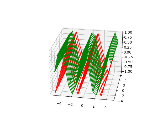
在这个例子中，我们将学习如何使用figure.gca()进行 3D 绘图。在这里，我们将创建一条正弦曲线和一条余弦曲线，x 和 y 的值范围为 -5 到 5，间隙为 1。让我们看一下代码以了解实现。

蟒蛇3

# importing matplotlib.pyplot from
# python
import matplotlib.pyplot as plt
 
# importing numpy package from
# python
import numpy as np
 
# creating a range of values for
# x,y,x1,y1  from -5 to 5 with
# a space of 1 between the elements
x = np.arange(-5,5,1)
y = np.arange(-5,5,1)
 
# creating a range of values for
# x,y,x1,y1  from -5 to 5 with
# a space of 0.6 between the elements
x1= np.arange(-5,5,0.6)
y1= np.arange(-5,5,0.6)
 
# Creating a mesh grid with x ,y and x1,
# y1 which creates an n-dimensional
# array
x, y = np.meshgrid(x, y)
x1,y1= np.meshgrid(x1,y1)
 
# Creating a sine function with the
# range of values from the meshgrid
z = np.sin(x * np.pi/2 )
 
# Creating a cosine function with the
# range of values from the meshgrid
z1= np.cos(x1* np.pi/2)
 
# Creating an empty figure for
# 3D plotting
fig = plt.figure()
 
# using fig.gca, we are creating a 3D
# projection plot in the empty figure
ax = fig.gca(projection="3d")
 
# Creating a wireframe plot with the x,y and
# z-coordinates respectively along with the
# color as red
surf = ax.plot_wireframe(x, y, z, color="red")
 
# Creating a wireframe plot with the points
# x1,y1,z1 along with the plot line as green
surf1 =ax.plot_wireframe(x1, y1, z1, color="green")
 
#showing the above plot
plt.show()

输出：

解释：

• 在这个例子中，我们导入了两个包matplotlib.pyplot 和来自Python 的NumPy 。
• 之后，我们使用各种变量（例如 x、y、x1、x2）创建范围广泛的值。现在这里有一个问题。第一组 x,y 具有从 -5 到 5 的值，每个元素彼此之间的差值为 1。第二组元素的范围也从 -5 到 5，每个元素彼此之间的差异为 0.6。它创建的不同之处在于，第一个图将具有陡峭的曲线，因为点之间的差异更大，而在第二组中，与第一个图相比，该图将更平滑，因为我们采用了广泛的点超过 x 和 y。这就是为什么第二条曲线（余弦曲线）比第一条曲线更平滑的原因。
• 使用meshgrid ，我们从坐标向量返回坐标矩阵。 MeshGrid制作 ND 坐标数组，用于对 ND 网格上的 ND 标量/矢量场进行矢量化评估，其中有一维数组。现在，我们分别在 z 和 z1 的帮助下创建正弦和余弦曲线。
• 之后，我们将创建一个空图形，我们将在其中绘制 3D 绘图。使用fig.gca，我们定义了我们将要制作的图将是使用projection='3d'的 3D 投影。使用plot_wireframe我们正在使用我们创建的上述点创建 3D 正弦和余弦曲线（不同颜色）。最后，我们展示了上面的图。

示例 3：

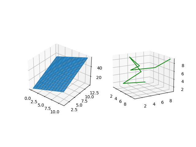
在最后一个也是最后一个示例中，我们将在单个图形/画布中创建两个 3D 图形，其中我们将成为我们的 3D 点。所以让我们进入我们的代码实现。

蟒蛇3

#importing matplotlib.pyplot from
# python
import matplotlib.pyplot as plt
 
# importing numpy package from python
import numpy as np
 
# creating an empty figure for plotting
fig = plt.figure()
 
# defining a sub-plot with 1x2 axis and defining
# it as first plot with projection as 3D
ax = fig.add_subplot(1, 2, 1, projection='3d')
 
# creating a range of 12 elements in both
# X and Y
X = np.arange(12)
Y = np.linspace(12, 1)
 
# Creating a mesh grid of X and Y
X, Y = np.meshgrid(X, Y)
 
# Creating an expression X and Y and
# storing it in Z
Z = X*2+Y*3;
 
# Creating a wireframe plot with the 3 sets of
# values X,Y and Z
ax.plot_wireframe(X, Y, Z)
 
# Creating my second subplot with 1x2 axis and defining
# it as the second plot with projection as 3D
ax = fig.add_subplot(1, 2, 2, projection='3d')
 
# defining a set of points for X,Y and Z
X1 = [1,2,1,4,3,2,7,5,9]
Y1 = [8,2,7,4,3,6,1,8,9]
Z1 = [1,2,4,7,9,6,7,6,9]
 
# Plotting 3 points X1,Y1,Z1 with
# color as green
ax.plot(X1, Y1, Z1,color='green')
 
# Showing the above plot
plt.show()

输出：

解释：

• 在上面的示例中，我们将使用 2 个 3D 图形。为此，我们将在单个画布或图形中创建两个子图。在代码中，我们初始化了包matplotlib.pyplot ， 和 NumPy 像往常一样来自Python 。
• 然后我们创建一个空图形，其中将绘制两个 3D 图。现在我们正在创建第一个子图。
• 在此之后，我们正在采取X，Y包含一系列点，并用它们，我们正在创建，其由两个一维二维阵列的向上和用于矩阵索引以创建ND阵列的meshgrid。
• 然后，使用 X 和 Y 的值，我们通过形成表达式来创建 Z。使用plot_wireframe我们在 3D 轴上绘制点。
• 之后，我们转到第二个图，在那里我们定义第二个子图参数。
• 然后，我们正在创建范围广泛的元素并将它们以数组的形式存储在 X1、Y1 和 Z1 中。
• 之后，我们使用上述点绘制图形，稍后我们将显示包含 2 个 3D 图形的图形。

使用 Matplotlib 的关键 3D 绘图：

 曲面图和三曲面图

在这里，我们将看看如何创建曲面图和三曲面图。在这里，我们将两个图整合到一个图中，以便我们可以理解子图的概念以及要绘制的各种点的图的概念。那么让我们开始实施这个概念。与线框图不同，这些图的表面将填充颜色。

例子：

蟒蛇3

#importing matplotlib.pyplot from
# python
import matplotlib.pyplot as plt
 
# importing numpy package from python
import numpy as np
 
# creating an empty figure for plotting
fig = plt.figure()
 
# defining a sub-plot with 1x2 axis and defining
# it as first plot with projection as 3D
ax = fig.add_subplot(1, 2, 1, projection='3d')
 
# creating a range of values for
# x1,y1  from -1 to 1 with
# a space of 0.1 between the elements so that
# we can create a single curve in the plot
x1= np.arange(-1,1,0.1)
y1= np.arange(-1,1,0.1)
 
# Creating a mesh grid with x ,y and x1,
# y1 which creates an n-dimensional
# array
x1,y1= np.meshgrid(x1,y1)
 
# Creating a cosine function with the
# range of values from the meshgrid
z1= np.cos(x1* np.pi/2)
 
# Creating a wireframe plot with the points
# x1,y1,z1 along with the plot line as red
ax.plot_surface(x1, y1, z1, color="red")
 
# Creating my second subplot with 1x2 axis and defining
# it as the second plot with projection as 3D
ax = fig.add_subplot(1, 2, 2, projection='3d')
 
# defining a set of points for X1,Y1 and Z1
X1 = [1,2,1,4,3,2,7,5,9]
Y1 = [8,2,7,4,3,6,1,8,9]
Z1 = [1,2,4,7,9,6,7,6,9]
 
# Plotting 3 points X1,Y1,Z1 with
# color as purple
ax.plot_trisurf(X1, Y1, Z1,color='purple')
 
# Showing the above plot
plt.show()

输出：

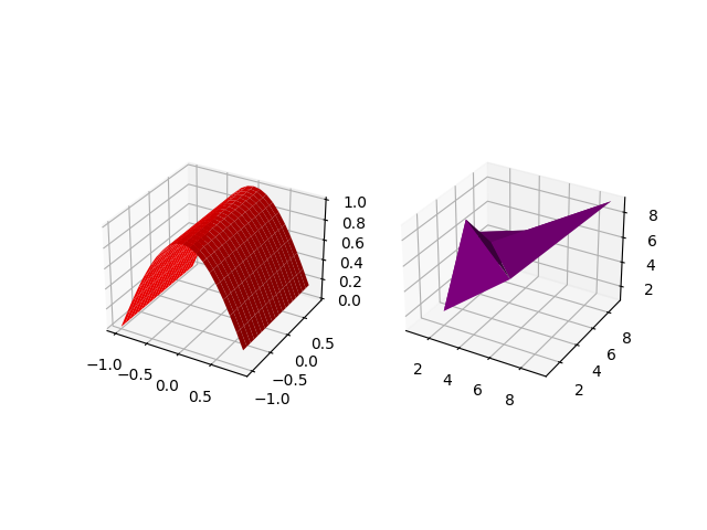
解释：

• 导入所有必要的包（ numpy ， matplotlib.pyplot ）后，我们正在使用plt.figure()创建一个空图，我们正在向上图中添加子图，其中我们将 1,2,1 作为参数以及投影作为 3D。这使我们能够创建一个 1×2 大小的图，我们将其定义为第一个图。
• 然后我们创建了从 -1 到 1 的范围很广的值，以 0.1 的差值均匀分布，并将它们存储在 x1 和 y1 中。
• 然后，使用meshgrid ，我们为 x1 和 y1 创建一个 nD 数组。
• 使用 x1 的值，我们正在创建一条余弦曲线并将值集存储在 z1 中。
• 在ax.plot_surface()的帮助下，我们绘制了一个定义 x1、y1 和 z1 点的曲面图，以及曲面图的颜色为红色。
• 之后，我们定义相同大小的第二个图，即 1×2，并将其定义为第二个图。我们使用变量 X1、Y1 和 Z1 来创建一组点并将它们存储在这些列表中。
• 使用ax.plot_trisurf()我们将 X1、Y1 和 Z1 的点和图形的颜色定义为紫色。最后，我们展示了上面的图。

等高线图和填充等高线图

在这里，我们将查看等高线图和填充等高线图。由于两个图的类型相似，我们再次使用子图来绘制点。等高线图是一种通过绘制恒定 z 切片来显示 3D 图形的方式。填充等高线填充等高线图中线条显示的区域。

蟒蛇3

# importing axes3d from mpl_toolkits.mplot
# module in python
from mpl_toolkits.mplot3d import axes3d
 
# importing matplotlib package from python
import matplotlib.pyplot as plt
 
#importing numpy package from
# python library
import numpy as np
 
# Creating an empty figure
fig = plt.figure()
 
# Creating a subplot where we are
# defining the projection as 3D projection
ax = fig.add_subplot(1,2,1, projection='3d')
 
# Creating a set of testing data using
# get_test_data from axes3d module in
# python. It creates a set of nD arrays
# for each of the variables X,Y,Z
X, Y, Z = axes3d.get_test_data(0.07)
#Plotting the contour plot with the
# following range of nD arrays
plot = ax.contour(X, Y, Z)
 
# Adding a second subplot in our figure with
# the projection as a 3D projection
ax=fig.add_subplot(1,2,2,projection='3d')
 
# Adding a range of values to the variables X1,Y1
X1=[1,2,3,4,5,6,7]
Y1=[1,2,3,4,5,6,7]
 
# Creating a meshgrid of X1 and Y1
X1, Y1 = np.meshgrid(X1,Y1)
# Creating an expression for Z1 with the
# help of X1 and Y1
Z1=(X1+4)*5+(Y1-5)/2
 
# Creating a contour plot
plot2 = ax.contourf(X1, Y1, Z1)
 
# Showing the above plot
plt.show()

输出：

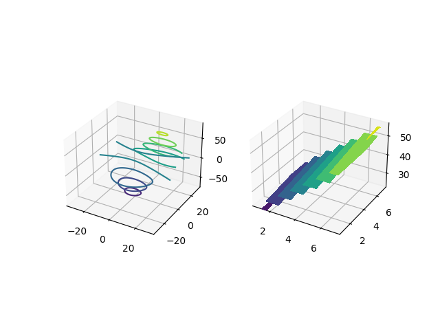
解释：

• 第一步是导入绘制上图所需的所有包。除了matplotlib.pyplot 和NumPy ，我们正在导入另一个包mpl_toolkits.mplot3d 。
• 之后，我们将创建一个空图形，我们将在其中放置 2 个 3D 子图。
• 之后，我们添加大小为 1×2 的第一个子图并定义第一个子图。
• 之后，我们使用 3 个变量，并在get_test_data的帮助下创建一个自动网格，这将帮助我们绘制图中的点。使用ax.contour(X,Y,Z) 我们正在创建一个具有以下值范围的等高线图。
• 之后，我们定义相同大小的第二个图。填充的等高线图 不需要meshgrid 。可以使用 X1、Y1、Z1 中的简单值范围创建它。 Z1 是在使用 X1 和 Y1 创建的表达式的帮助下形成的。使用ax.contourf(X1,Y1,Z1) 我们正在绘制一个填充的等高线图。
• 最后，我们展示了带有 2 个子图的上图。

多边形图

在这里，我们将探索多边形图。此图与前面示例中绘制的图不同。在此图中，我们将在 z 的不同轴点上绘制一组连续的点。让我们转向实施。

例子：

蟒蛇3

# import Axes3D from mpl_toolkits.mplot3d
# from python
from mpl_toolkits.mplot3d import Axes3D
 
# importing PolyCollection from
# matplotlib.collections module
from matplotlib.collections import PolyCollection
 
#importing matplotlib.pyplot from
# python
import matplotlib.pyplot as plt
 
# importing numpy package from
# python
import numpy as np
 
# Creating an empty figure
fig = plt.figure()
 
# Creating a 3D projection using
# fig.gca
ax = fig.gca(projection='3d')
 
# Creating a wide range of elements
# using numpy package from python
xs = np.arange(0, 1, 0.1)
# Creating an empty list
verts = []
# Creating a range of values on
# Z-Axis
zs = [0.0, 0.2, 0.4, 0.6,0.8]
# Looping through all the values in zs
# and creating random values in ys using
# np.random.rand() which creates a range of
# elements in ys and we are appending each of them
# inside verts[]
for z in zs:
    ys = np.random.rand(len(xs))
    verts.append(list(zip(xs, ys)))
# using polycollection, we are providing a
# series of vertices to poly so as to
# plot our required plot
poly = PolyCollection(verts)
# Using add_collection3d, we are plotting
# ur required ploygon plot where we define
# zs with the range of values we defined in our
# list zs and also the zdir as Y-Axis
ax.add_collection3d(poly,zs=zs,zdir='y')
# Showing the required plot
plt.show()

输出：

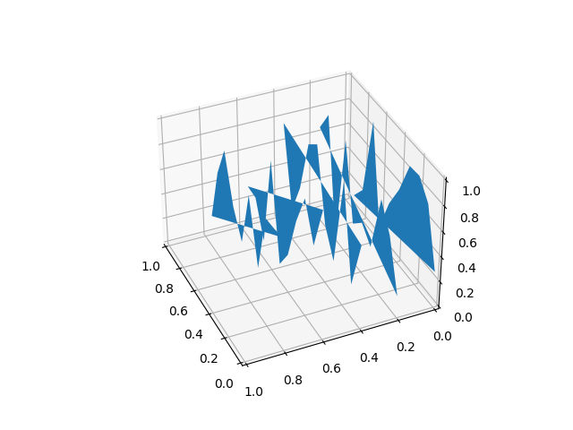
解释：

• 在这个例子中，我们需要导入 4 个不同的包来创建这个图（ Numpy、matplotlib.pyplot、polycollection、Axes3d ）。
• 之后，我们将创建一个空图，我们将在其中绘制上图。使用arange和一系列任意值，我们在 x 和 z 中创建了一个值列表。现在我们通过 z循环，其中对于 z 的每个值，我们将获得与x 的那个。
• 现在对于每个 z，我们正在沿线绘制 x 与 y。使用PolyCollection ，我们将每个图中的所有图都使用相同的颜色。在add_collection3d的帮助下，我们确定要在 xz 轴上绘制绘图并定义 zs=0。
• 最后，我们展示了上面的图。

箭袋图

在这里，我们将学习 matplotlib 中的箭袋图。箭袋图帮助我们绘制一个 3d 箭头区域以定义指定的点。我们可以通过各种方式自定义箭头。让我们看看代码实现。

例子：

蟒蛇3

# import axes3d from mpl_toolkits.mplot3d
from mpl_toolkits.mplot3d import axes3d
 
# import matplotlib.pyplot from python
import matplotlib.pyplot as plt
 
# import numoy from python
import numpy as np
 
# Creating an empty figure
# to plot a 3D graph
fig = plt.figure()
 
# Creating a 3Dprojection for
# our 3D plots using fig.gca
ax = fig.gca(projection='3d')
 
# Creating a meshgrid for the range
# of values in X,Y,Z
x, y, z = np.meshgrid([1,2,5,2,4,8,3,3,1],[6,4,3,1,6,2,7,8,2],[1,2,5,2,4,8,3,3,1])
 
# Creating expressions for u,v,w
# with the help of x,y and z
# which will form the direction vectors
u = x*2+y*3+z*3
v = (x+3)*(y+5)*(z+7)
w = x+y+z
 
# Creating a quiver plot with length of the direction
# vector length as 0.2 ad normalise as true
ax.quiver(x, y, z, u, v, w, length=0.2, normalize=True)
 
#showing the above plot
plt.show()

输出：

解释：

• 在上面的代码中，我们在顶部导入所有必要的包（ matplotlib.pyplot,numpy,mpl_toolkit.mplot3d ）。
• 然后我们在plt.figure()的帮助下创建一个空图形。在fig.gca(projection='3d')的帮助下，我们将投影指定为 3D，即 3D 绘图。
• 使用meshgrid，我们创建了一个包含X、Y 和Z 的ND 阵列。在箭袋图中，绘制点并不是唯一的任务。我们需要指定向量方向的分量。因此，为此，我们采用了 u、v、z，它们是通过使用 X、Y 和 Z 创建的不同表达式形成的。
• 使用ax.quiver()我们绘制箭袋图，其中我们将每个箭袋的长度指定为 0.1，为了使箭头具有相同的长度，我们将normalize定义为True 。

 要在 3D 图中绘制的 2D 数据

在这里，我们将在 3D 图中的特定轴上绘制一组 2D 点，因为我们无法在具有所有坐标的 3D 平面中绘制 2D 点。因此需要定义一个特定的轴来绘制 2D 点。那么让我们看看情节的代码。

蟒蛇3

# importing numpy package
import numpy as np
# importing matplotlib package
import matplotlib.pyplot as plt
 
# Creating an empty canvas(figure)
fig = plt.figure()
 
# Using the gca function, we are defining
# the current axes as a 3D projection
ax = fig.gca(projection='3d')
 
# Labelling X-Axis
ax.set_xlabel('X-Axis')
 
# Labelling Y-Axis
ax.set_ylabel('Y-Axis')
 
# Labelling Z-Axis
ax.set_zlabel('Z-Axis')
 
# Creating 10 values for X
x = [1,1.2,1.4,1.6,1.8,2.0,2.2,2.4,2.6,2.8]
 
# Creating 10 values for Y
y = [1,1.2,1.4,1.6,1.8,2.0,2.2,2.4,2.6,2.8]
 
# Creating 10 random values for Y
z=[1,2,4,5,6,7,8,9,10,11]
 
# zdir='z' fixes all the points to zs=0 and
# (x,y) points are ploted in the x-y axis
# of the graph
ax.plot(x, y, zs=0, zdir='z')
 
# zdir='y' fixes all the points to zs=0 and
# (x,y) points are ploted in the x-z axis of the
# graph
ax.plot(x, y, zs=0, zdir='y')
 
# Showing the above plot
plt.show()

输出：

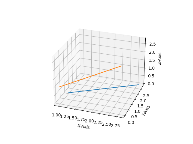
解释：

• 在此示例中，我们将在 Matplotlib 中的 3D 绘图上绘制 2D 数据。为此，我们需要NumPy和matplotlib.pyplot来创建一组值并在 3D 投影中绘制它们。导入所有必要的包后，我们将在 X、Y 和 Z 中创建范围广泛的值。
• 现在在ax.plot()的帮助下，我们正在绘制我们的 2D 点，我们将要绘制的两个集合指定为ax.plot() 中的参数以及它们要绘制的轴。