R 编程中的偏度和峰度

在统计学中，偏度和峰度是描述数据分布形状的度量，或者简单地说，两者都是分析数据集形状的数值方法，不像绘制图形和直方图是图形方法。这些是用于检查分布的不规则性和不对称性的正态性检验。要在 R 语言中计算偏度和峰度，需要moment包。

偏度

偏度是一种统计数值方法，用于测量分布或数据集的不对称性。它讲述了大多数数据值在平均值周围的分布中的位置。
公式：
${\displaystyle \gamma_{1}=\frac{\frac{1}{n} \sum_{i=1}^{n}\left(x_{i}-\bar{x}\right)^{3}}{\left(\frac{1}{n} \sum_{i=1}^{n}\left(x_{i}-\bar{x}\right)^{2}\right)^{3 / 2}}}$
在哪里，

$<strong>\gamma_{1} </strong>$represents coefficient of skewness 
$<strong>x_{i} </strong>$represents $i^\text{th}$value in data vector 
$<strong>\bar{x} </strong>$represents mean of data vector 
n represents total number of observations

存在 3 种偏度值，根据这些偏度值来确定图形的不对称性。这些如下：

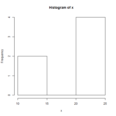
正偏斜

如果偏度系数大于 0 即$\gamma_{1}>0$ ，则该图被认为是正偏斜的，大多数数据值小于均值。大多数值都集中在图表的左侧。
例子：

Python3

# Required for skewness() function
library(moments)
 
# Defining data vector
x <- c(40, 41, 42, 43, 50)
 
# output to be present as PNG file
png(file = "positiveskew.png")
 
# Print skewness of distribution
print(skewness(x))
 
# Histogram of distribution
hist(x)
 
# Saving the file
dev.off()

输出：

[1] 1.2099

图示：

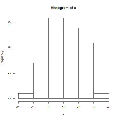
零偏度或对称

如果偏度系数等于 0 或近似接近 0，即$\gamma_{1}=0$ ，则称该图是对称的，并且数据是正态分布的。
例子：

Python3

# Required for skewness() function
library(moments)
 
# Defining normally distributed data vector
x <- rnorm(50, 10, 10)
 
# output to be present as PNG file
png(file = "zeroskewness.png")
 
# Print skewness of distribution
print(skewness(x))
 
# Histogram of distribution
hist(x)
 
# Saving the file
dev.off()

输出：

[1] -0.02991511

图示：

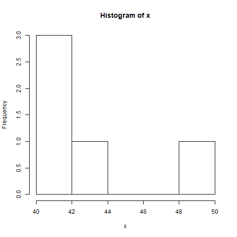
负偏斜

如果偏度系数小于 0 即$\gamma_{1}<0$ ，则该图被称为负偏斜，大多数数据值大于均值。大多数值都集中在图表的右侧。
例子：

Python3

# Required for skewness() function
library(moments)
 
# Defining data vector
x <- c(10, 11, 21, 22, 23, 25)
 
# output to be present as PNG file
png(file = "negativeskew.png")
 
# Print skewness of distribution
print(skewness(x))
 
# Histogram of distribution
hist(x)
 
# Saving the file
dev.off()

输出：

[1] -0.5794294

图示：

峰度

峰度是统计学中的一种数值方法，用于测量数据分布中峰值的锐度。
公式：
${\displaystyle \gamma_{2}=\frac{\frac{1}{n} \sum_{i=1}^{n}\left(x_{i}-\bar{x}\right)^{4}}{\left(\frac{1}{n} \sum_{i=1}^{n}\left(x_{i}-\bar{x}\right)^{2}\right)^{2}} }$
在哪里，

$<strong>\gamma_{2} </strong>$represents coefficient of kurtosis 
$<strong>x_{i} </strong>$represents $i^\text{th}$value in data vector 
$<strong>\bar{x} </strong>$represents mean of data vector 
n represents total number of observations

存在 3 种类型的峰度值，在此基础上测量峰的锐度。这些如下：

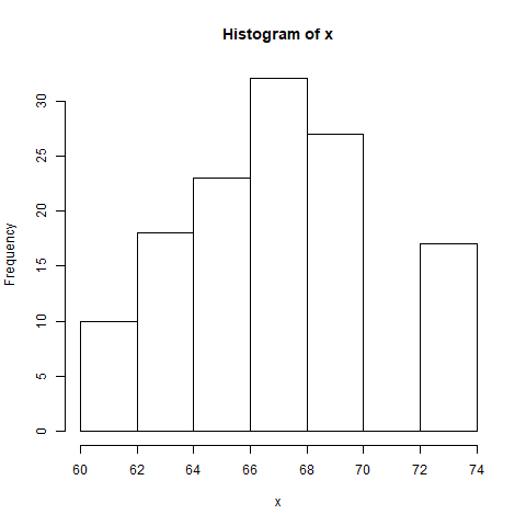
桔梗

如果峰度系数小于 3 即$\gamma_{2}<3$ ，则数据分布为 platykurtic。 platykurtic 并不意味着图表是平顶的。
例子：

Python3

# Required for kurtosis() function
library(moments)
 
# Defining data vector
x <- c(rep(61, each = 10), rep(64, each = 18),
rep(65, each = 23), rep(67, each = 32), rep(70, each = 27),
rep(73, each = 17))
 
# output to be present as PNG file
png(file = "platykurtic.png")
 
# Print skewness of distribution
print(kurtosis(x))
 
# Histogram of distribution
hist(x)
 
# Saving the file
dev.off()

输出：

[1] 2.258318

图示：

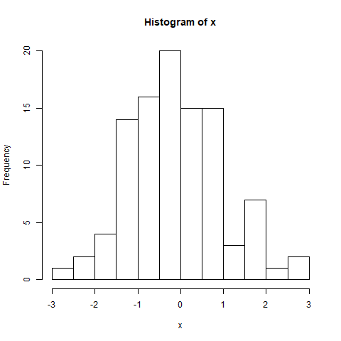
中峰

如果峰度系数等于 3 或接近 3，即$\gamma_{2}=3$ ，则数据分布是中峰的。对于正态分布，峰度值大约等于 3。
例子：

Python3

# Required for kurtosis() function
library(moments)
 
# Defining data vector
x <- rnorm(100)
 
# output to be present as PNG file
png(file = "mesokurtic.png")
 
# Print skewness of distribution
print(kurtosis(x))
 
# Histogram of distribution
hist(x)
 
# Saving the file
dev.off()

输出：

[1] 2.963836

图示：

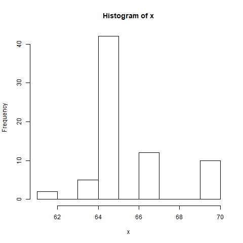
尖峰

如果峰度系数大于 3 即$\gamma_{1}>3$ ，则数据分布呈尖峰形，并在图上显示一个尖峰。
例子：

Python3

# Required for kurtosis() function
library(moments)
 
# Defining data vector
x <- c(rep(61, each = 2), rep(64, each = 5),
rep(65, each = 42), rep(67, each = 12), rep(70, each = 10))
 
# output to be present as PNG file
png(file = "leptokurtic.png")
 
# Print skewness of distribution
print(kurtosis(x))
 
# Histogram of distribution
hist(x)
 
# Saving the file
dev.off()

输出：

[1] 3.696788

图示：