最大流量的 Dinic 算法
问题陈述 :
给定一个表示流网络的图,其中每条边都有容量。还给定图中的两个顶点 source 's' 和 sink 't',找到从 s 到 t 的最大可能流,具有以下约束:
- 边缘上的流量不超过边缘的给定容量。
- 除了 s 和 t 之外,每个顶点的流入流等于流出流。
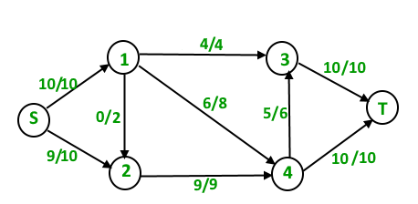
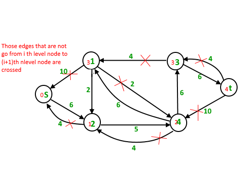
例如,在下面的输入图中,

最大 st 流量为 19,如下所示。
背景 :
- 最大流量问题介绍:我们介绍了最大流量问题,讨论了贪心算法并介绍了残差图。
- Ford-Fulkerson 算法和 Edmond Karp 实现:我们讨论了 Ford-Fulkerson 算法及其实现。我们还详细讨论了残差图。
Edmond Karp 实现的时间复杂度为 O(VE 2 )。在这篇文章中,讨论了一种新的 Dinic 算法,它是一种更快的算法并且需要 O(EV 2 )。
与 Edmond Karp 的算法一样,Dinic 的算法使用以下概念:
- 如果残差图中没有s到t路径,则流是最大的。
- BFS 在循环中使用。尽管我们在两种算法中使用 BFS 的方式有所不同。
在 Edmond 的 Karp 算法中,我们使用 BFS 来查找增广路径并通过该路径发送流量。在 Dinic 的算法中,我们使用 BFS 来检查是否有更多的流是可能的,并构建水平图。在级别图中,我们为所有节点分配级别,节点的级别是节点到源的最短距离(就边数而言)。一旦构建了级别图,我们就使用此级别图发送多个流。这就是它比 Edmond Karp 工作得更好的原因。在 Edmond Karp 中,我们只发送通过 BFS 找到的路径发送的流。
Dinic 算法概述:
1) Initialize residual graph G as given graph.
1) Do BFS of G to construct a level graph (or
   assign levels to vertices) and also check if
   more flow is possible.
    a) If more flow is not possible, then return.
    b) Send multiple flows in G using level graph
       until blocking flow is reached. Here using
       level graph means, in every flow,
       levels of path nodes should be 0, 1, 2...
(in order) from s to t.如果无法使用级别图发送更多流,则流是阻塞流,即不存在更多路径,因此路径顶点按顺序具有当前级别 0、1、2……。阻塞流可以看作与此处讨论的贪心算法中的最大流路相同。
插图 :
初始残差图(与给定图相同)
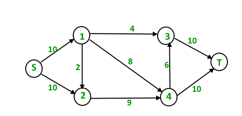
总流量 = 0
第一次迭代:我们使用 BFS 为所有节点分配级别。我们还检查是否可能有更多的流量(或者残差图中有一个 st 路径)。
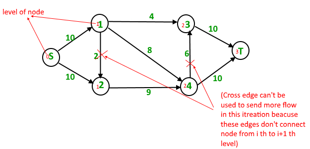
现在我们使用级别找到阻塞流(意味着每个流路径的级别应该为 0、1、2、3)。我们一起发送三个流。与我们一次发送一个流的 Edmond Karp 相比,这是优化的地方。
路径 s – 1 – 3 – t 上的 4 个单位流量。
路径 s – 1 – 4 – t 上的 6 个单位流量。
路径 s – 2 – 4 – t 上的 4 个单位流量。
总流量 = 总流量 + 4 + 6 + 4 = 14
一次迭代后,残差图变为以下。
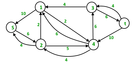
第二次迭代:我们使用上述修改残差图的 BFS 为所有节点分配新级别。我们还检查是否可能有更多的流量(或者残差图中有一个 st 路径)。
现在我们使用级别找到阻塞流(意味着每个流路径的级别应该为 0、1、2、3、4)。这次我们只能发送一个流。
路径 s – 2 – 4 – 3 – t 上的 5 个单位流量
总流量 = 总流量 + 5 = 19
新的残差图是
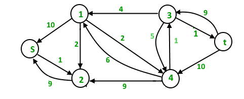
第三次迭代:我们运行 BFS 并创建一个级别图。我们还会检查是否有更多流量,并且仅在可能的情况下继续。这次残差图中没有 st 路径,所以我们终止算法。
执行 :
下面是 Dinic 算法的 c++ 实现:
CPP
// C++ implementation of Dinic's Algorithm
#include
using namespace std;

// A structure to represent a edge between
// two vertex
struct Edge
{
    int v ;  // Vertex v (or "to" vertex)
             // of a directed edge u-v. "From"
             // vertex u can be obtained using
             // index in adjacent array.

    int flow ; // flow of data in edge

    int C;    // capacity

    int rev ; // To store index of reverse
              // edge in adjacency list so that
              // we can quickly find it.
};

// Residual Graph
class Graph
{
    int V; // number of vertex
    int *level ; // stores level of a node
    vector< Edge > *adj;
public :
    Graph(int V)
    {
        adj = new vector[V];
        this->V = V;
        level = new int[V];
    }

    // add edge to the graph
    void addEdge(int u, int v, int C)
    {
        // Forward edge : 0 flow and C capacity
        Edge a{v, 0, C, adj[v].size()};

        // Back edge : 0 flow and 0 capacity
        Edge b{u, 0, 0, adj[u].size()};

        adj[u].push_back(a);
        adj[v].push_back(b); // reverse edge
    }

    bool BFS(int s, int t);
    int sendFlow(int s, int flow, int t, int ptr[]);
    int DinicMaxflow(int s, int t);
};

// Finds if more flow can be sent from s to t.
// Also assigns levels to nodes.
bool Graph::BFS(int s, int t)
{
    for (int i = 0 ; i < V ; i++)
        level[i] = -1;

    level[s] = 0;  // Level of source vertex

    // Create a queue, enqueue source vertex
    // and mark source vertex as visited here
    // level[] array works as visited array also.
    list< int > q;
    q.push_back(s);

    vector::iterator i ;
    while (!q.empty())
    {
        int u = q.front();
        q.pop_front();
        for (i = adj[u].begin(); i != adj[u].end(); i++)
        {
            Edge &e = *i;
            if (level[e.v] < 0  && e.flow < e.C)
            {
                // Level of current vertex is,
                // level of parent + 1
                level[e.v] = level[u] + 1;

                q.push_back(e.v);
            }
        }
    }

    // IF we can not reach to the sink we
    // return false else true
    return level[t] < 0 ? false : true ;
}

// A DFS based function to send flow after BFS has
// figured out that there is a possible flow and
// constructed levels. This function called multiple
// times for a single call of BFS.
// flow : Current flow send by parent function call
// start[] : To keep track of next edge to be explored.
//           start[i] stores  count of edges explored
//           from i.
//  u : Current vertex
//  t : Sink
int Graph::sendFlow(int u, int flow, int t, int start[])
{
    // Sink reached
    if (u == t)
        return flow;

    // Traverse all adjacent edges one -by - one.
    for (  ; start[u] < adj[u].size(); start[u]++)
    {
        // Pick next edge from adjacency list of u
        Edge &e = adj[u][start[u]];

        if (level[e.v] == level[u]+1 && e.flow < e.C)
        {
            // find minimum flow from u to t
            int curr_flow = min(flow, e.C - e.flow);

            int temp_flow = sendFlow(e.v, curr_flow, t, start);

            // flow is greater than zero
            if (temp_flow > 0)
            {
                // add flow  to current edge
                e.flow += temp_flow;

                // subtract flow from reverse edge
                // of current edge
                adj[e.v][e.rev].flow -= temp_flow;
                return temp_flow;
            }
        }
    }

    return 0;
}

// Returns maximum flow in graph
int Graph::DinicMaxflow(int s, int t)
{
    // Corner case
    if (s == t)
        return -1;

    int total = 0;  // Initialize result

    // Augment the flow while there is path
    // from source to sink
    while (BFS(s, t) == true)
    {
        // store how many edges are visited
        // from V { 0 to V }
        int *start = new int[V+1] {0};

        // while flow is not zero in graph from S to D
        while (int flow = sendFlow(s, INT_MAX, t, start))

            // Add path flow to overall flow
            total += flow;
    }

    // return maximum flow
    return total;
}

// Driver Code
int main()
{
    Graph g(6);
    g.addEdge(0, 1, 16 );
    g.addEdge(0, 2, 13 );
    g.addEdge(1, 2, 10 );
    g.addEdge(1, 3, 12 );
    g.addEdge(2, 1, 4 );
    g.addEdge(2, 4, 14);
    g.addEdge(3, 2, 9 );
    g.addEdge(3, 5, 20 );
    g.addEdge(4, 3, 7 );
    g.addEdge(4, 5, 4);

    // next exmp
    /*g.addEdge(0, 1, 3 );
      g.addEdge(0, 2, 7 ) ;
      g.addEdge(1, 3, 9);
      g.addEdge(1, 4, 9 );
      g.addEdge(2, 1, 9 );
      g.addEdge(2, 4, 9);
      g.addEdge(2, 5, 4);
      g.addEdge(3, 5, 3);
      g.addEdge(4, 5, 7 );
      g.addEdge(0, 4, 10);

     // next exp
     g.addEdge(0, 1, 10);
     g.addEdge(0, 2, 10);
     g.addEdge(1, 3, 4 );
     g.addEdge(1, 4, 8 );
     g.addEdge(1, 2, 2 );
     g.addEdge(2, 4, 9 );
     g.addEdge(3, 5, 10 );
     g.addEdge(4, 3, 6 );
     g.addEdge(4, 5, 10 ); */

    cout << "Maximum flow " << g.DinicMaxflow(0, 5);
    return 0;
}
输出:
Maximum flow 23时间复杂度: O(EV 2 )。使用 BFS 构建级别图需要 O(E) 时间。在到达阻塞流之前发送多个流需要 O(VE) 时间。外循环最多运行 O(V) 时间。在每次迭代中,我们构建新的级别图并找到阻塞流。可以证明,每一次迭代,层数至少增加一个(证明见下面的参考视频)。所以外循环最多运行 O(V) 次。因此总体时间复杂度为 O(EV 2 )。