KL 散度在变分自编码器中的作用

变分自编码器

变分自编码器由谷歌和高通公司的 Knigma 和 Welling 于 2013 年提出。变分自编码器 (VAE) 提供了一种概率方式来描述潜在空间中的观察。因此，与其构建一个输出单个值来描述每个潜在状态属性的编码器，我们将制定我们的编码器来描述每个潜在属性的概率分布。

建筑学：

自编码器基本上包含两部分：

• 第一个是编码器，除了最后一层外，与卷积神经网络类似。编码器的目标是从数据集中学习有效的数据编码并将其传递到瓶颈架构中。
• 自编码器的另一部分是解码器，它使用瓶颈层中的潜在空间来重新生成与数据集相似的图像。这些结果以损失函数的形式从神经网络反向传播。

变分自编码器与自编码器的不同之处在于它提供了一种统计方式来描述潜在空间中的数据集样本。因此，在变分自编码器中，编码器在瓶颈层输出概率分布而不是单个输出值。

解释：

变分自编码器潜在空间是连续的。它提供随机采样和插值。编码器输出两个向量，而不是输出大小为 n 的向量：

• 矢量？？？均值（向量大小 n）
• 矢量？？？标准偏差（向量大小 n）

输出是近似后验分布 q(z|x)。从这个分布中采样得到 z。让我们看看采样的更多细节：

• 让我们取一些平均值和标准差的值，
  • $\mu = [0.15, 1.1, 0.2, 0.7, ...] \\ \sigma =[0.2, 0.4, 0.5, 2.4, ...]$
• 从中生成的中间分布：
  • $X =[X_1 \sim \bold{N} (0.15, 0.2^2), X_2 \sim \bold{N} (1.1, 0,4^2), X_3 \sim \bold{N} (0.2, 0,5^2), X_4 \sim \bold{N} (0.7, 1.5^2), ...]$
• 现在，让我们从中生成采样向量：
  • $[0.32, 1.25, 0.8,2.0]$
• 虽然一个输入的均值和标准差相同，但结果可能因采样而不同。
• 最终，我们的目标是让编码器学会以不同的方式生成？？？对于不同的类，对它们进行聚类并生成编码，这样它们的差异不大。为此，我们使用 KL 散度。

KL-散度：

KL 散度代表 Kullback Leibler Divergence，它是两个分布之间散度的度量。我们的目标是最小化 KL 散度并优化 ????和 ？？？？一种分布以类似于所需的分布。

对于多重分布，KL散度可以计算为以下公式：

$\frac{1}{2}\sum_{j=1}^{J} (1 + log(\sigma_{j}^{(i)}))\frac{1}{2}\sum_{j=1}^{J} (1 + log(\sigma_{j}^{(i)})^{2}) -(\mu_j^{(i)})^{2} - (\sigma_j^{(i)})^{2})$

其中 X_j \sim N(\mu_j, \sigma_j^{2}) 是标准正态分布。

VAE 损失：

假设我们有一个分布 z 并且我们想从中生成观测值 x。换句话说，我们要计算

$p\left( {z|x} \right)$

我们可以通过以下方式做到：

$p\left( {z|x} \right) = \frac{{p\left( {x|z} \right)p\left( z \right)}}{{p\left( x \right)}}$

但是，p(x) 的计算可能相当困难

$p\left( x \right) = \int {p\left( {x|z} \right)p\left(z\right)dz}$

这通常使它成为一个难以处理的分布。因此，我们需要将 p(z|x) 近似为 q(z|x) 以使其成为易于处理的分布。为了更好地将 p(z|x) 逼近 q(z|x)，我们将最小化 KL 散度损失，计算两个分布的相似程度：

$\min KL\left( {q\left( {z|x} \right)||p\left( {z|x} \right)} \right)$

通过简化，上面的最小化问题等价于下面的最大化问题：

${E_{q\left( {z|x} \right)}}\log p\left( {x|z} \right) - KL\left( {q\left( {z|x} \right)||p\left( z \right)} \right)$

第一项代表重建可能性，另一项确保我们学习到的分布 q 与真实的先验分布 p 相似。

因此，我们的总损失由两项组成，一项是重构误差，另一项是 KL 散度损失：
$Loss = L\left( {x, \hat x} \right) + \sum\limits_j {KL\left( {{q_j}\left( {z|x} \right)||p\left( z \right)} \right)}$

执行：

在这个实现中，我们将使用 MNIST 数据集，这个数据集已经在keras.datasets API 中可用，所以我们不需要手动添加或上传。

• 首先，我们需要将必要的包导入到我们的Python环境中。我们将使用带有 TensorFlow 的 Keras 包作为后端。

python3

# code
import numpy as np
import tensorflow as tf
from tensorflow import keras
from tensorflow.keras import Input, Model
from tensorflow.keras.layers import Layer, Conv2D, Flatten, Dense, Reshape, Conv2DTranspose
import matplotlib.pyplot as plt

• 对于变分自编码器，我们需要定义编码器和解码器两部分的架构，但首先，我们将定义架构的瓶颈层，即采样层。

蟒蛇3

# this sampling layer is the bottleneck layer of variational autoencoder,
# it uses the output from two dense layers z_mean and z_log_var as input, 
# convert them into normal distribution and pass them to the decoder layer
class Sampling(Layer):
  
    def call(self, inputs):
        z_mean, z_log_var = inputs
        batch = tf.shape(z_mean)[0]
        dim = tf.shape(z_mean)[1]
        epsilon = tf.keras.backend.random_normal(shape =(batch, dim))
        return z_mean + tf.exp(0.5 * z_log_var) * epsilon

• 现在，我们定义自动编码器的编码器部分的架构，这部分将图像作为输入并在采样层中对其表示进行编码。

蟒蛇3

# Define Encoder Model
latent_dim = 2
  
encoder_inputs = Input(shape =(28, 28, 1))
x = Conv2D(32, 3, activation ="relu", strides = 2, padding ="same")(encoder_inputs)
x = Conv2D(64, 3, activation ="relu", strides = 2, padding ="same")(x)
x = Flatten()(x)
x = Dense(16, activation ="relu")(x)
z_mean = Dense(latent_dim, name ="z_mean")(x)
z_log_var = Dense(latent_dim, name ="z_log_var")(x)
z = Sampling()([z_mean, z_log_var])
encoder = Model(encoder_inputs, [z_mean, z_log_var, z], name ="encoder")
encoder.summary()

Model: "encoder"
__________________________________________________________________________________________________
Layer (type)                    Output Shape         Param #     Connected to                     
==================================================================================================
input_3 (InputLayer)            [(None, 28, 28, 1)]  0                                            
__________________________________________________________________________________________________
conv2d_2 (Conv2D)               (None, 14, 14, 32)   320         input_3[0][0]                    
__________________________________________________________________________________________________
conv2d_3 (Conv2D)               (None, 7, 7, 64)     18496       conv2d_2[0][0]                   
__________________________________________________________________________________________________
flatten_1 (Flatten)             (None, 3136)         0           conv2d_3[0][0]                   
__________________________________________________________________________________________________
dense_2 (Dense)                 (None, 16)           50192       flatten_1[0][0]                  
__________________________________________________________________________________________________
z_mean (Dense)                  (None, 2)            34          dense_2[0][0]                    
__________________________________________________________________________________________________
z_log_var (Dense)               (None, 2)            34          dense_2[0][0]                    
__________________________________________________________________________________________________
sampling_1 (Sampling)           (None, 2)            0           z_mean[0][0]                     
                                                                 z_log_var[0][0]                  
==================================================================================================
Total params: 69, 076
Trainable params: 69, 076
Non-trainable params: 0
__________________________________________________________________________________________________

• 现在，我们定义自动编码器的解码器部分的架构，这部分以采样层的输出作为输入并输出大小为 (28, 28, 1) 的图像。  

蟒蛇3

# Define Decoder Architecture
latent_inputs = keras.Input(shape =(latent_dim, ))
x = Dense(7 * 7 * 64, activation ="relu")(latent_inputs)
x = Reshape((7, 7, 64))(x)
x = Conv2DTranspose(64, 3, activation ="relu", strides = 2, padding ="same")(x)
x = Conv2DTranspose(32, 3, activation ="relu", strides = 2, padding ="same")(x)
decoder_outputs = Conv2DTranspose(1, 3, activation ="sigmoid", padding ="same")(x)
decoder = Model(latent_inputs, decoder_outputs, name ="decoder")
decoder.summary()

Model: "decoder"
_________________________________________________________________
Layer (type)                 Output Shape              Param #   
=================================================================
input_4 (InputLayer)         [(None, 2)]               0         
_________________________________________________________________
dense_3 (Dense)              (None, 3136)              9408      
_________________________________________________________________
reshape_1 (Reshape)          (None, 7, 7, 64)          0         
_________________________________________________________________
conv2d_transpose_3 (Conv2DTr (None, 14, 14, 64)        36928     
_________________________________________________________________
conv2d_transpose_4 (Conv2DTr (None, 28, 28, 32)        18464     
_________________________________________________________________
conv2d_transpose_5 (Conv2DTr (None, 28, 28, 1)         289       
=================================================================
Total params: 65, 089
Trainable params: 65, 089
Non-trainable params: 0
_________________________________________________________________

• 在这一步中，我们结合模型并使用损失函数定义训练过程。  

蟒蛇3

# this class takes encoder and decoder models and
# define the complete variational autoencoder architecture
class VAE(keras.Model):
    def __init__(self, encoder, decoder, **kwargs):
        super(VAE, self).__init__(**kwargs)
        self.encoder = encoder
        self.decoder = decoder
  
    def train_step(self, data):
        if isinstance(data, tuple):
            data = data[0]
        with tf.GradientTape() as tape:
            z_mean, z_log_var, z = encoder(data)
            reconstruction = decoder(z)
            reconstruction_loss = tf.reduce_mean(
                keras.losses.binary_crossentropy(data, reconstruction)
            )
            reconstruction_loss *= 28 * 28
            kl_loss = 1 + z_log_var - tf.square(z_mean) - tf.exp(z_log_var)
            kl_loss = tf.reduce_mean(kl_loss)
            kl_loss *= -0.5
            # beta =10
            total_loss = reconstruction_loss + 10 * kl_loss
        grads = tape.gradient(total_loss, self.trainable_weights)
        self.optimizer.apply_gradients(zip(grads, self.trainable_weights))
        return {
            "loss": total_loss,
            "reconstruction_loss": reconstruction_loss,
            "kl_loss": kl_loss,
        }

• 现在是训练我们的变分自编码器模型的好时机，我们将训练它 100 个 epoch。但首先我们需要导入 MNIST 数据集。

蟒蛇3

# load fashion mnist dataset  from  keras.dataset API
(x_train, _), (x_test, _) = keras.datasets.fashion_mnist.load_data()
fmnist_images = np.concatenate([x_train, x_test], axis = 0)
# expand dimension to add  a color map dimension
fmnist_images = np.expand_dims(fmnist_images, -1).astype("float32") / 255
  
# compile and train the model
vae = VAE(encoder, decoder)
vae.compile(optimizer ='rmsprop')
vae.fit(fmnist_images, epochs = 100, batch_size = 128)

• 在这一步中，我们显示训练结果，我们将根据它们在潜在空间向量中的值来显示这些结果。

蟒蛇3

def plot_latent(encoder, decoder):
    # display a n * n 2D manifold of imagess
    n = 10
    img_dim = 28
    scale = 2.0
    figsize = 15
    figure = np.zeros((img_dim * n, img_dim * n))
    # linearly spaced coordinates corresponding to the 2D plot
    # of images classes in the latent space
    grid_x = np.linspace(-scale, scale, n)
    grid_y = np.linspace(-scale, scale, n)[::-1]
  
    for i, yi in enumerate(grid_y):
        for j, xi in enumerate(grid_x):
            z_sample = np.array([[xi, yi]])
            x_decoded = decoder.predict(z_sample)
            images = x_decoded[0].reshape(img_dim, img_dim)
            figure[
                i * img_dim : (i + 1) * img_dim,
                j * img_dim : (j + 1) * img_dim,
            ] = images
  
    plt.figure(figsize =(figsize, figsize))
    start_range = img_dim // 2
    end_range = n * img_dim + start_range + 1
    pixel_range = np.arange(start_range, end_range, img_dim)
    sample_range_x = np.round(grid_x, 1)
    sample_range_y = np.round(grid_y, 1)
    plt.xticks(pixel_range, sample_range_x)
    plt.yticks(pixel_range, sample_range_y)
    plt.xlabel("z[0]")
    plt.ylabel("z[1]")
    plt.imshow(figure, cmap ="Greys_r")
    plt.show()
  
  
plot_latent(encoder, decoder)

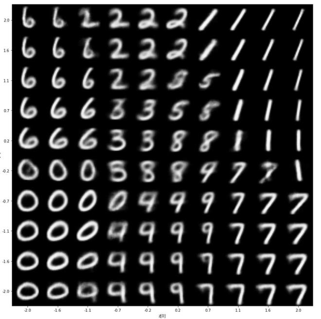
编码器输出

• 为了更清楚地了解我们的代表性潜在向量值，我们将根据编码器生成的相应潜在维度的值绘制训练数据的散点图 

蟒蛇3

def plot_label_clusters(encoder, decoder, data, test_lab):
    z_mean, _, _ = encoder.predict(data)
    plt.figure(figsize =(12, 10))
    sc = plt.scatter(z_mean[:, 0], z_mean[:, 1], c = test_lab)
    cbar = plt.colorbar(sc, ticks = range(10))
    cbar.ax.set_yticklabels([i for i in range(10)])
    plt.xlabel("z[0]")
    plt.ylabel("z[1]")
    plt.show()
  
(x_train, y_train), _ = keras.datasets.mnist.load_data()
x_train = np.expand_dims(x_train, -1).astype("float32") / 255
plot_label_clusters(encoder, decoder, x_train, y_train)

Beta 的分布 = 10

• 为了比较差异，我还为 \beta =0 训练了上述自动编码器，即我们去除了 Kl-divergence 损失，并且它生成了以下分布：

Beta = 0 的分布

在这里，我们可以看到分布不可分离并且对于不同的值非常偏斜，这就是我们在上述变分自编码器中使用 KL 散度损失的原因。

参考：

• 变分自编码器论文
• Keras 变分自动编码器