毫升 |使用Python 的多元线性回归

线性回归：
它是预测分析的基本和常用类型。它是一种对因变量和一组给定的自变量之间的关系进行建模的统计方法。

它们有两种类型：

简单线性回归
多元线性回归

让我们使用Python讨论多元线性回归。

多元线性回归尝试通过将线性方程拟合到观测数据来模拟两个或多个特征与响应之间的关系。执行多重线性回归的步骤几乎与简单线性回归的步骤相似。区别在于评价。我们可以用它来找出哪个因素对预测输出的影响最大，现在不同的变量相互关联。

Here : Y = b0 + b1 * x1 + b2 * x2 + b3 * x3 + …… bn * xn
Y = Dependent variable and x1, x2, x3, …… xn = multiple independent variables

编程需要懂一点英语

回归模型假设：

线性：因变量和自变量之间的关系应该是线性的。
同方差性：应保持误差的恒定方差。
多元正态性：多元回归假设残差呈正态分布。
缺乏多重共线性：假设数据中很少或没有多重共线性。

虚拟变量 -
正如我们在多重回归模型中所知，我们使用了大量分类数据。使用分类数据是将非数字数据包含到各自的回归模型中的好方法。类别数据是指表示类别数据值的数据值，具有固定和无序数量的值，例如性别（男性/女性）。在回归模型中，这些值可以用虚拟变量来表示。

这些变量由 0 或 1 等值组成，代表分类值的存在和不存在。

虚拟变量陷阱 –
虚拟变量陷阱是两个或多个高度相关的情况。简单来说，我们可以说一个变量可以从另一个变量的预测中得到预测。虚拟变量陷阱的解决方案是删除一个分类变量。因此，如果有m 个虚拟变量，则在模型中使用m-1 个变量。

D2 = D1-1   
 Here D2, D1 = Dummy Variables

建造模型的方法：

全押
向后消除
前向选择
双向消除
分数比较

向后消除：

第 1 步：选择一个重要级别以在模型中开始。
第 2 步：用所有可能的预测器拟合完整模型。
第 3 步：考虑具有最高 P 值的预测器。如果 P > SL 转到步骤 4，否则模型准备就绪。
第 4 步：删除预测器。
第 5 步：拟合没有此变量的模型。

前向选择：

第 1 步：选择一个显着性水平以输入模型（例如 SL = 0.05）
第 2 步：拟合所有简单回归模型 y~x(n)。选择 P 值最低的那个。
第 3 步：保留这个变量并拟合所有可能的模型，并在您已有的模型中添加一个额外的预测器。
第 4 步：考虑具有最低 P 值的预测器。如果 P < SL，转到步骤 #3，否则模型准备就绪。

任何多元线性回归模型中涉及的步骤

第 1 步：数据预处理

导入库。
导入数据集。
编码分类数据。
避免虚拟变量陷阱。
将数据集拆分为训练集和测试集。

第 2 步：将多元线性回归拟合到训练集
第 3 步：预测测试集结果。

代码 1：

import numpy as np
import matplotlib as mpl
from mpl_toolkits.mplot3d import Axes3D
import matplotlib.pyplot as plt
  
def generate_dataset(n):
    x = []
    y = []
    random_x1 = np.random.rand()
    random_x2 = np.random.rand()
    for i in range(n):
        x1 = i
        x2 = i/2 + np.random.rand()*n
        x.append([1, x1, x2])
        y.append(random_x1 * x1 + random_x2 * x2 + 1)
    return np.array(x), np.array(y)
  
x, y = generate_dataset(200)
  
mpl.rcParams['legend.fontsize'] = 12
  
fig = plt.figure()
ax = fig.gca(projection ='3d')
  
ax.scatter(x[:, 1], x[:, 2], y, label ='y', s = 5)
ax.legend()
ax.view_init(45, 0)
  
plt.show()

输出：

代码 2：

def mse(coef, x, y):
    return np.mean((np.dot(x, coef) - y)**2)/2
  
def gradients(coef, x, y):
    return np.mean(x.transpose()*(np.dot(x, coef) - y), axis = 1)
  
def multilinear_regression(coef, x, y, lr, b1 = 0.9, b2 = 0.999, epsilon = 1e-8):
    prev_error = 0
    m_coef = np.zeros(coef.shape)
    v_coef = np.zeros(coef.shape)
    moment_m_coef = np.zeros(coef.shape)
    moment_v_coef = np.zeros(coef.shape)
    t = 0
  
    while True:
        error = mse(coef, x, y)
        if abs(error - prev_error) <= epsilon:
            break
        prev_error = error
        grad = gradients(coef, x, y)
        t += 1
        m_coef = b1 * m_coef + (1-b1)*grad
        v_coef = b2 * v_coef + (1-b2)*grad**2
        moment_m_coef = m_coef / (1-b1**t)
        moment_v_coef = v_coef / (1-b2**t)
  
        delta = ((lr / moment_v_coef**0.5 + 1e-8) * 
                 (b1 * moment_m_coef + (1-b1)*grad/(1-b1**t)))
  
        coef = np.subtract(coef, delta)
    return coef
  
coef = np.array([0, 0, 0])
c = multilinear_regression(coef, x, y, 1e-1)
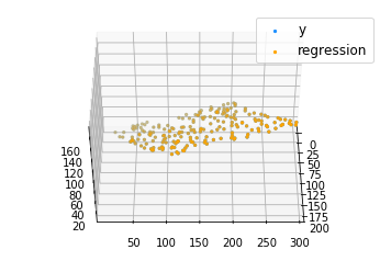
fig = plt.figure()
ax = fig.gca(projection ='3d')
  
ax.scatter(x[:, 1], x[:, 2], y, label ='y',
                s = 5, color ="dodgerblue")
  
ax.scatter(x[:, 1], x[:, 2], c[0] + c[1]*x[:, 1] + c[2]*x[:, 2],
                    label ='regression', s = 5, color ="orange")
  
ax.view_init(45, 0)
ax.legend()
plt.show()

输出：