R中的时间序列分析

R 中的时间序列用于查看对象在一段时间内的行为。在 R 中，可以通过带有一些参数的ts()函数轻松完成。时间序列采用数据向量，每个数据都与用户给定的时间戳值连接。该函数主要用于学习和预测资产在一段时间内的业务行为。例如，公司的销售分析、库存分析、特定股票或市场的价格分析、人口分析等。

Syntax:  objectName <- ts(data, start, end, frequency)

where,

• data represents the data vector
• start represents the first observation in time series
• end represents the last observation in time series
• frequency represents number of observations per unit time. For example, frequency=1 for monthly data.

注意：要了解更多可选参数，请在 R 控制台中使用以下命令：

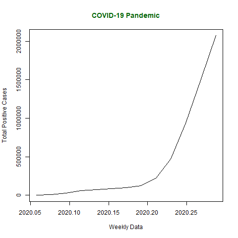
help("ts")

示例：让我们以 COVID-19 大流行情况为例。从 2020 年 1 月 22 日到 2020 年 4 月 15 日，每周在数据向量中获取全球 COVID-19 阳性病例总数。

R

# Weekly data of COVID-19 positive cases from
# 22 January, 2020 to 15 April, 2020
x <- c(580, 7813, 28266, 59287, 75700,
    87820, 95314, 126214, 218843, 471497,
    936851, 1508725, 2072113)
 
# library required for decimal_date() function
library(lubridate)
 
# output to be created as png file
png(file ="timeSeries.png")
 
# creating time series object
# from date 22 January, 2020
mts <- ts(x, start = decimal_date(ymd("2020-01-22")),
                            frequency = 365.25 / 7)
 
# plotting the graph
plot(mts, xlab ="Weekly Data",
        ylab ="Total Positive Cases",
        main ="COVID-19 Pandemic",
        col.main ="darkgreen")
 
# saving the file
dev.off()

输出：

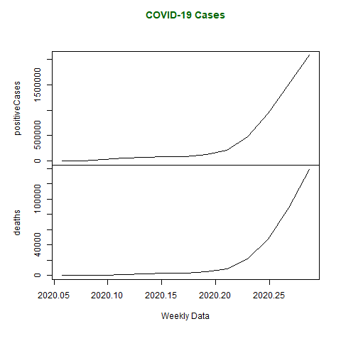
多元时间序列

多元时间序列在单个图表中创建多个时间序列。

示例：从 2020 年 1 月 22 日到 2020 年 4 月 15 日，每周在数据向量中获取 COVID-19 的阳性病例总数和死亡总数数据。

R

# Weekly data of COVID-19 positive cases and
# weekly deaths from 22 January, 2020 to
# 15 April, 2020
positiveCases <- c(580, 7813, 28266, 59287,
                75700, 87820, 95314, 126214,
                218843, 471497, 936851,
                1508725, 2072113)
 
deaths <- c(17, 270, 565, 1261, 2126, 2800,
            3285, 4628, 8951, 21283, 47210,
            88480, 138475)
 
# library required for decimal_date() function
library(lubridate)
 
# output to be created as png file
png(file ="multivariateTimeSeries.png")
 
# creating multivariate time series object
# from date 22 January, 2020
mts <- ts(cbind(positiveCases, deaths),
start = decimal_date(ymd("2020-01-22")),
                    frequency = 365.25 / 7)
 
# plotting the graph
plot(mts, xlab ="Weekly Data",
    main ="COVID-19 Cases",
    col.main ="darkgreen")
 
# saving the file
dev.off()

输出：

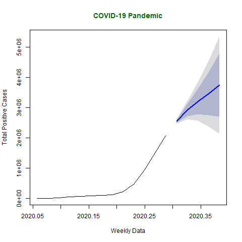
预测

可以使用 R 中存在的一些模型对时间序列进行预测。在此示例中，使用了 Arima 自动模型。要了解 arima()函数的更多参数，请使用以下命令。

help("arima")

在下面的代码中，预测是使用预测库完成的，因此需要安装预测库。

R

# Weekly data of COVID-19 cases from
# 22 January, 2020 to 15 April, 2020
x <- c(580, 7813, 28266, 59287, 75700,
    87820, 95314, 126214, 218843,
    471497, 936851, 1508725, 2072113)
 
# library required for decimal_date() function
library(lubridate)
 
# library required for forecasting
library(forecast)
 
# output to be created as png file
png(file ="forecastTimeSeries.png")
 
# creating time series object
# from date 22 January, 2020
mts <- ts(x, start = decimal_date(ymd("2020-01-22")),
                            frequency = 365.25 / 7)
 
# forecasting model using arima model
fit <- auto.arima(mts)
 
# Next 5 forecasted values
forecast(fit, 5)
 
# plotting the graph with next
# 5 weekly forecasted values
plot(forecast(fit, 5), xlab ="Weekly Data",
ylab ="Total Positive Cases",
main ="COVID-19 Pandemic", col.main ="darkgreen")
 
# saving the file
dev.off()

输出 ：
执行上述代码后，会产生以下预测结果。

Point Forecast   Lo 80   Hi 80   Lo 95   Hi 95
2020.307        2547989 2491957 2604020 2462296 2633682
2020.326        2915130 2721277 3108983 2618657 3211603
2020.345        3202354 2783402 3621307 2561622 3843087
2020.364        3462692 2748533 4176851 2370480 4554904
2020.383        3745054 2692884 4797225 2135898 5354210

下图绘制了 COVID-19 在未来 5 周内继续广泛传播时的估计预测值。