如何使用 ggplot2 在 R 中绘制碎石图

在本文中，我们将了解如何使用 ggplot2 在 R 编程语言中绘制 Scree 图。

加载数据集：

在这里我们将加载数据集，（记得去掉非数字列）。由于鸢尾花数据集包含一个字符类型的物种列，因此我们需要删除它，因为PCA仅适用于数值数据。

R

# drop the species column as its character type
num_iris = subset(iris,
                  select = -c(Species))
head(num_iris)

输出：

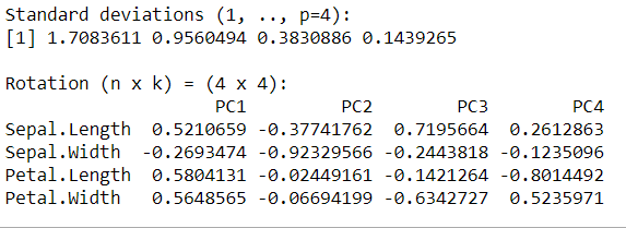
使用prcomp ()函数计算主成分分析

我们使用 R 语言内置的 prcomp()函数，该函数将数据集作为参数并计算PCA 。主成分分析 (PCA) 是一种统计过程，它使用正交变换将一组相关变量转换为一组不相关变量。做scale=TRUE标准化数据。

Syntax: prcomp(numeric_data, scale = TRUE)

代码：

电阻

# drop the species column as its character type
num_iris = subset(iris, select = -c(Species) )
 
# compute pca
pca <- prcomp(num_iris, scale = TRUE)
pca

输出：

计算每个主成分解释的方差：

我们使用下面的公式来计算每台 PC 所经历的总方差。

Syntax: pca$sdev^2 / sum(pca$sdev^2)

代码：

电阻

# drop the species column as its character type
num_iris = subset(iris, select = -c(Species) )
 
# compute pca
pca <- prcomp(num_iris, scale = TRUE)
 
# compute total variance
variance = pca$sdev^2 / sum(pca$sdev^2)
variance

输出：

[1] 0.729624454 0.228507618 0.036689219 0.005178709

示例 1：使用线图绘制碎石图

电阻

library(ggplot2)
 
# drop the species column as its character type
num_iris = subset(iris, select = -c(Species) )
 
# compute pca
pca <- prcomp(num_iris, scale = TRUE)
 
# compute total variance
variance = pca $sdev^2 / sum(pca $sdev^2)
 
# Scree plot
qplot(c(1:4), variance) +
  geom_line() +
  geom_point(size=4)+
  xlab("Principal Component") +
  ylab("Variance Explained") +
  ggtitle("Scree Plot") +
  ylim(0, 1)

输出：

示例 2 ：使用条形图绘制碎石图

电阻

library(ggplot2)
 
# drop the species column as its character type
num_iris = subset(iris, select = -c(Species) )
 
# compute pca
pca <- prcomp(num_iris, scale = TRUE)
 
# compute total variance
variance = pca $sdev^2 / sum(pca $sdev^2)
 
# Scree plot
qplot(c(1:4), variance) +
  geom_col()+
  xlab("Principal Component") +
  ylab("Variance Explained") +
  ggtitle("Scree Plot") +
  ylim(0, 1)

输出：