在 R 中绘制 t 分布

t 分布，也称为学生 t 分布，是一种概率分布，用于对样本量很小且输入分布的标准偏差未知的正态分布进行抽样。分布通常形成钟形曲线，即分布呈正态分布，但峰值较低，尾部附近的观测值较多。

t 分布只有一个相关参数，称为自由度 (df)。特定 t 分布曲线的形状取决于所选的自由度 (df) 的数量，该数量等于给定的样本量减 1，即，

df=n−1

可以使用 R 中的 seq() 方法生成坐标向量，该方法用于生成整数的增量序列，为给定的 t 分布提供分布序列。可以使用下面详述的 t 分布函数的各种变体来构建相应的 y 坐标。然后使用 R 编程语言中的 plot() 方法绘制这些图。

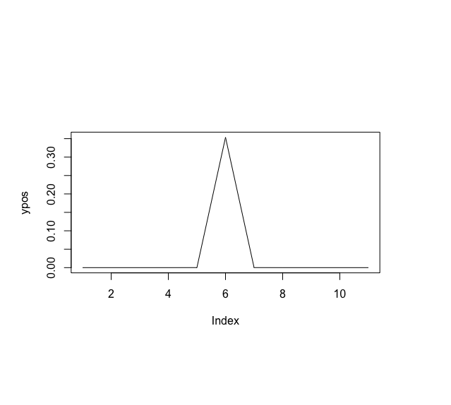
dt() 方法

R 中的 dt() 方法用于计算具有指定自由度的 t 分布的概率密度分析。

Syntax:

dt(x, df )

Parameter : 

• x – vector of quantiles
• df – degrees of freedom

例子：

R

# generating x coordinates
xpos <- seq(- 100, 100, by = 20) 
 
print ("X coordinates")
print (xpos)
 
# generating y coordinates using dt() method
# degreesoffreedom
degree <- 2
ypos <- dt(xpos, df = degree)
 
print ("Y coordinates")
print (ypos)
 
# plotting t distribution
plot (ypos , type = "l")

输出

[1] “X coordinates” 

[1] -100  -80  -60  -40  -20    0   20   40   60   80  100

[1] “Y coordinates” 

[1] 9.997001e-07 1.952210e-06 4.625774e-06 1.559575e-05 1.240683e-04  [6] 3.535534e-01 1.240683e-04 1.559575e-05 4.625774e-06 1.952210e-06 

[11] 9.997001e-07

pt() 方法

R 中的 pt() 方法用于为给定的学生 T 分布生成分布函数。它用于产生累积分布函数。此函数返回任何给定间隔的 t 曲线下的面积。

Syntax:

pt(q, df, lower.tail = TRUE)

Parameter : 

• q – quantile vector
• df – degrees of freedom
• lower.tail – if TRUE (default), probabilities are P[X ≤ x], otherwise, P[X > x].

例子：

电阻

# generating x coordinates
xpos <- seq(- 100, 100, by = 20) 
 
print ("X coordinates")
print (xpos)
 
# generating y coordinates using dt() method
# degreesoffreedom
degree <- 2
 
ypos <- pt(xpos, df = degree)
 
print ("Y coordinates")
print (ypos)
 
# plotting t distribution
plot (ypos , type = "l")

输出

[1] “X coordinates” 

[1] -100  -80  -60  -40  -20    0   20   40   60   80  100 

[1] “Y coordinates” 

[1] 4.999250e-05 7.810669e-05 1.388310e-04 3.122073e-04 1.245332e-03  [6] 5.000000e-01 9.987547e-01 9.996878e-01 9.998612e-01 9.999219e-01 

[11] 9.999500e-01

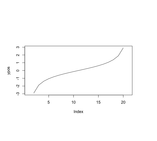
qt() 方法

R 中的 qt() 方法用于计算指定数量自由度的给定 t 分布的分位数函数或逆累积密度函数。它用于计算具有指定自由度的学生 t 分布的第 n 个百分位数。

Syntax:

qt(p, df, lower.tail = TRUE)

Parameter : 

• p – vector of probabilities
• df – degrees of freedom
• lower.tail – if TRUE (default), probabilities are P[X ≤ x], otherwise, P[X > x].

例子：

电阻

# generating x coordinates
xpos <- seq(0, 1, by = 0.05)
 
# generating y coordinates using dt() method
# degreesoffreedom
degree <- 2
ypos <- qt(xpos, df = degree)
 
# plotting t distribution
plot (ypos , type = "l")

输出

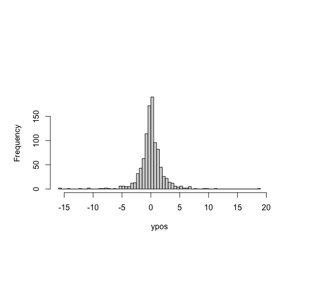
rt() 方法

rt() 方法用于使用指定数量的自由度随机生成 t 分布。可以生成 n 个随机样本。

Syntax:

rt(n, df)

Parameter : 

• n – number of observations
• df – degrees of freedom

例子：

电阻

# using a random number
n <- 1000
 
# degreesoffreedom
degree <- 2
 
# generating y coordinates using rt() method
ypos <- rt(n , df = degree)
 
# plotting t distribution in the form of
# distribution
hist(ypos,                                       
     breaks = 100,
     main = "")

输出