在 R 编程中使用 k-Nearest Neighbors 进行回归
机器学习是人工智能的一个子集,它为机器提供了无需明确编程即可自动学习的能力。在这种情况下,机器在没有人为干预的情况下从经验中改进,并相应地调整动作。它主要有3种类型:
- 监督机器学习
- 无监督机器学习
- 强化学习
K-最近邻
K-最近邻算法创建一个假想的边界来对数据进行分类。当添加新数据点进行预测时,算法会将该点添加到最近的边界线。它遵循“物以类聚”的原则。该算法可以很容易地用 R 语言实现。
K-NN 算法
- 选择 K,邻居的数量。
- 计算 K 个邻居的欧几里得距离。
- 根据计算的欧几里得距离取 K 个最近邻。
- 计算这 K 个邻居中每个类别的数据点数。
- 新数据点被分配给邻居数量最大的类别。
R中的实现
数据集: 400 人的样本人口与一家产品公司分享了他们的年龄、性别和薪水,以及他们是否购买了该产品(0 表示否,1 表示是)。下载数据集 Advertisement.csv
R
# Importing the dataset
dataset = read.csv('Advertisement.csv')
head(dataset, 10)
R
# Encoding the target
# feature as factor
dataset$Purchased = factor(dataset$Purchased,
                           levels = c(0, 1))

# Splitting the dataset into
# the Training set and Test set
# install.packages('caTools')
library(caTools)
set.seed(123)
split = sample.split(dataset$Purchased,
                     SplitRatio = 0.75)
training_set = subset(dataset,
                      split == TRUE)
test_set = subset(dataset,
                  split == FALSE)

# Feature Scaling
training_set[-3] = scale(training_set[-3])
test_set[-3] = scale(test_set[-3])

# Fitting K-NN to the Training set
# and Predicting the Test set results
library(class)
y_pred = knn(train = training_set[, -3],
             test = test_set[, -3],
             cl = training_set[, 3],
             k = 5,
             prob = TRUE)

# Making the Confusion Matrix
cm = table(test_set[, 3], y_pred)
R
# Visualising the Training set results
# Install ElemStatLearn if not present
# in the packages using(without hashtag)
# install.packages('ElemStatLearn')
library(ElemStatLearn)
set = training_set
#Building a grid of Age Column(X1)
# and Estimated Salary(X2) Column
X1 = seq(min(set[, 1]) - 1,
max(set[, 1]) + 1,
by = 0.01)
X2 = seq(min(set[, 2]) - 1,
max(set[, 2]) + 1,
by = 0.01)
grid_set = expand.grid(X1, X2)
# Give name to the columns of matrix
colnames(grid_set) = c('Age',
'EstimatedSalary')
# Predicting the values and plotting
# them to grid and labelling the axes
y_grid = knn(train = training_set[, -3],
test = grid_set,
cl = training_set[, 3],
k = 5)
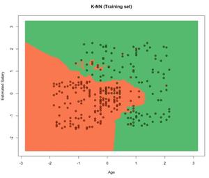
plot(set[, -3],
main = 'K-NN (Training set)',
xlab = 'Age', ylab = 'Estimated Salary',
xlim = range(X1), ylim = range(X2))
contour(X1, X2, matrix(as.numeric(y_grid),
length(X1), length(X2)),
add = TRUE)
points(grid_set, pch = '.',
col = ifelse(y_grid == 1,
'springgreen3', 'tomato'))
points(set, pch = 21, bg = ifelse(set[, 3] == 1,
'green4', 'red3'))R
# Visualising the Test set results
library(ElemStatLearn)
set = test_set
# Building a grid of Age Column(X1)
# and Estimated Salary(X2) Column
X1 = seq(min(set[, 1]) - 1,
max(set[, 1]) + 1,
by = 0.01)
X2 = seq(min(set[, 2]) - 1,
max(set[, 2]) + 1,
by = 0.01)
grid_set = expand.grid(X1, X2)
# Give name to the columns of matrix
colnames(grid_set) = c('Age',
'EstimatedSalary')
# Predicting the values and plotting
# them to grid and labelling the axes
y_grid = knn(train = training_set[, -3],
test = grid_set,
cl = training_set[, 3], k = 5)
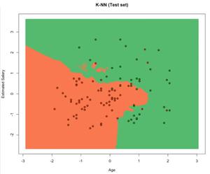
plot(set[, -3],
main = 'K-NN (Test set)',
xlab = 'Age', ylab = 'Estimated Salary',
xlim = range(X1), ylim = range(X2))
contour(X1, X2, matrix(as.numeric(y_grid),
length(X1), length(X2)),
add = TRUE)
points(grid_set, pch = '.', col =
ifelse(y_grid == 1,
'springgreen3', 'tomato'))
points(set, pch = 21, bg =
ifelse(set[, 3] == 1,
'green4', 'red3'))输出:
| User ID | Gender | Age | EstimatedSalary | Purchased | |
| 0 | 15624510 | Male | 19 | 19000 | 0 |
| 1 | 15810944 | Male | 35 | 20000 | 0 |
| 2 | 15668575 | Female | 26 | 43000 | 0 |
| 3 | 15603246 | Female | 27 | 57000 | 0 |
| 4 | 15804002 | Male | 19 | 76000 | 0 |
| 5 | 15728773 | Male | 27 | 58000 | 0 |
| 6 | 15598044 | Female | 27 | 84000 | 0 |
| 7 | 15694829 | Female | 32 | 150000 | 1 |
| 8 | 15600575 | Male | 25 | 33000 | 0 |
| 9 | 15727311 | Female | 35 | 65000 | 0 |
R
# Encoding the target
# feature as factor
dataset$Purchased = factor(dataset$Purchased,
                           levels = c(0, 1))

# Splitting the dataset into
# the Training set and Test set
# install.packages('caTools')
library(caTools)
set.seed(123)
split = sample.split(dataset$Purchased,
                     SplitRatio = 0.75)
training_set = subset(dataset,
                      split == TRUE)
test_set = subset(dataset,
                  split == FALSE)

# Feature Scaling
training_set[-3] = scale(training_set[-3])
test_set[-3] = scale(test_set[-3])

# Fitting K-NN to the Training set
# and Predicting the Test set results
library(class)
y_pred = knn(train = training_set[, -3],
             test = test_set[, -3],
             cl = training_set[, 3],
             k = 5,
             prob = TRUE)

# Making the Confusion Matrix
cm = table(test_set[, 3], y_pred)
- 训练集包含 300 个条目。
- 测试集包含 100 个条目。
Confusion matrix result:
[[64][4]
  [3][29]]
可视化训练数据:
R
# Visualising the Training set results
# Install ElemStatLearn if not present
# in the packages using(without hashtag)
# install.packages('ElemStatLearn')
library(ElemStatLearn)
set = training_set

#Building a grid of Age Column(X1)
# and Estimated Salary(X2) Column
X1 = seq(min(set[, 1]) - 1,
         max(set[, 1]) + 1,
         by = 0.01)
X2 = seq(min(set[, 2]) - 1,
         max(set[, 2]) + 1,
         by = 0.01)
grid_set = expand.grid(X1, X2)

# Give name to the columns of matrix
colnames(grid_set) = c('Age',
                       'EstimatedSalary')

# Predicting the values and plotting
# them to grid and labelling the axes
y_grid = knn(train = training_set[, -3],
             test = grid_set,
             cl = training_set[, 3],
             k = 5)
plot(set[, -3],
     main = 'K-NN (Training set)',
     xlab = 'Age', ylab = 'Estimated Salary',
     xlim = range(X1), ylim = range(X2))
contour(X1, X2, matrix(as.numeric(y_grid),
                       length(X1), length(X2)),
                       add = TRUE)
points(grid_set, pch = '.',
       col = ifelse(y_grid == 1,
                    'springgreen3', 'tomato'))
points(set, pch = 21, bg = ifelse(set[, 3] == 1,
                                  'green4', 'red3'))
输出:
可视化测试数据:
R
# Visualising the Test set results
library(ElemStatLearn)
set = test_set

# Building a grid of Age Column(X1)
# and Estimated Salary(X2) Column
X1 = seq(min(set[, 1]) - 1,
         max(set[, 1]) + 1,
         by = 0.01)
X2 = seq(min(set[, 2]) - 1,
         max(set[, 2]) + 1,
         by = 0.01)
grid_set = expand.grid(X1, X2)

# Give name to the columns of matrix
colnames(grid_set) = c('Age',
                       'EstimatedSalary')

# Predicting the values and plotting
# them to grid and labelling the axes
y_grid = knn(train = training_set[, -3],
             test = grid_set,
             cl = training_set[, 3], k = 5)
plot(set[, -3],
     main = 'K-NN (Test set)',
     xlab = 'Age', ylab = 'Estimated Salary',
     xlim = range(X1), ylim = range(X2))
contour(X1, X2, matrix(as.numeric(y_grid),
                       length(X1), length(X2)),
                       add = TRUE)
points(grid_set, pch = '.', col =
       ifelse(y_grid == 1,
              'springgreen3', 'tomato'))
points(set, pch = 21, bg =
       ifelse(set[, 3] == 1,
              'green4', 'red3'))
输出:
好处
- 没有培训期。
- KNN 是一种基于实例的学习算法,因此是一种惰性学习器。
- KNN 没有从训练表中导出任何判别函数,也没有训练周期。
- KNN 存储训练数据集并使用它进行实时预测。
- 新数据可以无缝添加,不会影响算法的准确性,因为新添加的数据不需要训练。
- 实现KNN算法只需要两个参数,即K值和欧几里得距离函数。
缺点
- 在新数据集中计算每个现有点与新点之间的距离的成本是巨大的,这降低了算法的性能。
- 算法很难计算每个维度的距离,因为该算法不适用于高维数据,即具有大量特征的数据,
- 在将 KNN 算法应用于任何数据集之前,需要进行特征缩放(标准化和规范化),否则 KNN 可能会生成错误的预测。
- KNN 对数据中的噪声很敏感。