如何处理散景中的图像

在本文中，我们将了解如何在 Bokeh 中处理图像。

为此，我们将使用ImageURL Glyph 。此字形呈现从给定 URL 加载的图像。

Syntax: ImageURL(‘url’, ‘x’, ‘y’, ‘w’, ‘h’, ‘angle’, ‘dilate’)

Arguments:

url: The url from where the images needs to be retrieved.
x = NumberSpec(default=field(“x”), the x-coordinates to locate the image anchors.
y = NumberSpec(default=field(“y”), the y-coordinates to locate the image anchors.
w = NullDistanceSpec, the width of the plot region that the image will occupy in data space.The default value is “None“, in which case the image will be displayed at its actual image size.
h = NullDistanceSpec, the height of the plot region that the image will occupy in data space.The default value is “None“, in which case the image will be displayed at its actual image size (regardless of the units specified here).
angle = AngleSpec(default=0), the angles with which the images are to be rotated, as measured from the horizontal.
global_alpha = Float(1.0), an overall opacity that each image is rendered with.
dilate = Bool(False), Whether to always round fractional pixel locations in such a way as to make the images bigger.This setting may be useful if pixel rounding errors are causing images to have a gap between them, when they should appear flush.
anchor = Enum(Anchor), What position of the image should be anchored at the `x`, `y` coordinates.
retry_attempts = Int(0), number of attempts to retry loading the images from the specified URL. Default is zero.
retry_timeout = Int(0), timeout (in ms) between retry attempts to load the image from the specified URL. Default is zero ms.

编程需要懂一点英语

示例 1：从 URL 导入图像

在这个例子中，我们从给定的 URL 加载图像，然后在绘图上渲染图像。在此示例中，我们从 Web 加载图像，该图像也可以在本地加载。在这里，我们在绘图上显示了两个具有不同参数值（例如 x、y、w、h 等）的图像。您可以观察输出以更好地理解。

Python

# importing numpy package and other libraries
import numpy as np
from bokeh.io import curdoc, show
from bokeh.models import ColumnDataSource, Grid, ImageURL, LinearAxis, Plot, Range1d
from bokeh.plotting import figure
  
# url to load image from
url = "https://media.geeksforgeeks.org/wp-content/\
uploads/20210829161730/logo.png"
  
N = 5
  
# creating columndatasource
source = ColumnDataSource(dict(
    url=[url]*N,
    x1=np.arange(N),
    y1=np.arange(N),
    w1=[35]*N,
    h1=[64]*N,
))
  
# creating x and y axis range
xdr = Range1d(start=-100, end=300)
ydr = Range1d(start=-100, end=300)
  
# creating a plot with above x and y axes range
plot = Plot(
    title=None, x_range=xdr, y_range=ydr,
  plot_width=400, plot_height=400,
    min_border=0, toolbar_location=None)
  
# loading the image using imageUrl
image = ImageURL(url=["https://media.geeksforgeeks.org/\
wp-content/uploads/20210829161730/logo.png"],
                 x=50, y=80, w=200, h=250, anchor="bottom_left")
image1 = ImageURL(url="url", x="x1", y="y1", w="w1",
                  h="h1", anchor="center")
  
# rendering the images to the plot
plot.add_glyph(source, image)
plot.add_glyph(source, image1)
  
xaxis = LinearAxis()
plot.add_layout(xaxis, 'below')
  
yaxis = LinearAxis()
plot.add_layout(yaxis, 'left')
  
# adding grid lines to the plot
plot.add_layout(Grid(dimension=0, ticker=xaxis.ticker,
                     grid_line_color='#00ff00'))
  
plot.add_layout(Grid(dimension=1, ticker=yaxis.ticker,
                     grid_line_color='#00ff00'))
  
# creates output file
curdoc().add_root(plot)
curdoc().theme = 'caliber'
  
# showing the plot on output file
show(plot)

Python

# importing numpy package and other libraries
import numpy as np
from bokeh.io import curdoc, show
from bokeh.models import ColumnDataSource, Grid, ImageURL, LinearAxis, Plot, Range1d
from bokeh.plotting import figure
  
# create dict as basis for ColumnDataSource
data = {'x1': [10, 20, 30, 40, 50],
        'y1': [60, 70, 80, 90, 100]}
  
# create ColumnDataSource based on dict
source = ColumnDataSource(data=data)
  
# creating figure
p = figure(plot_height=500, plot_width=500)
p.circle(x="x1", y="y1", size=20, source=source)
  
# rendering the image using imageUrl
image = ImageURL(url=["https://media.geeksforgeeks.org/\
wp-content/uploads/20210902155548/imgurl2-200x112.jpg"],
                 x=80, y=100, w=50, h=40, anchor="center", 
                 retry_attempts=2)
  
# adding the images to the plot
p.add_glyph(source, image)
  
# creates output file
curdoc().add_root(p)
  
# showing the plot on output file
show(p)

输出：

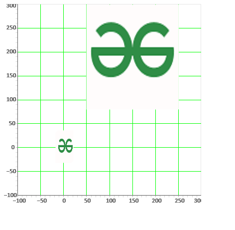
解释：

我们正在创建 ColumnDataSource，它为我们的绘图的字形提供数据。 Bokeh 有自己的数据结构，称为 ColumnDataSource，可用作任何 Bokeh 对象的输入。我们正在使用 NumPy 数组创建数据。
现在使用 range1d 创建 x 和 y 范围，它在标量维度中创建一个范围，然后将其分配给我们将在创建绘图时使用的 xdr 和 ydr。
然后我们用 xdr 和 ydr 作为 x_range 和 y_range 创建绘图，并将绘图的高度和宽度设置为 400。
然后，我们通过设置代码中所示的所有参数的值，从我们之前声明的 URL 中检索图像。我们通过给出不同的值在这里使用两个图像。
现在，我们将图像渲染到绘图中。
接下来，我们使用 Grid函数将网格线添加到绘图中，并为其指定颜色“绿色”。
然后，我们将绘图添加到应用程序代码 curdoc 中，它代表一个新文档并发送到 bokehJs 以将其显示给用户。

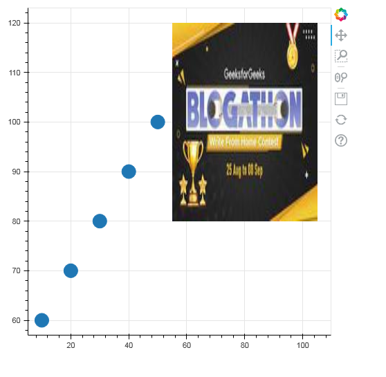
示例 2：创建圆形字形

在此示例中，我们将创建一个带有圆形字形的图形，然后使用字形 ImageURL 简单地从给定的 URL 渲染图像。

Python

# importing numpy package and other libraries
import numpy as np
from bokeh.io import curdoc, show
from bokeh.models import ColumnDataSource, Grid, ImageURL, LinearAxis, Plot, Range1d
from bokeh.plotting import figure
  
# create dict as basis for ColumnDataSource
data = {'x1': [10, 20, 30, 40, 50],
        'y1': [60, 70, 80, 90, 100]}
  
# create ColumnDataSource based on dict
source = ColumnDataSource(data=data)
  
# creating figure
p = figure(plot_height=500, plot_width=500)
p.circle(x="x1", y="y1", size=20, source=source)
  
# rendering the image using imageUrl
image = ImageURL(url=["https://media.geeksforgeeks.org/\
wp-content/uploads/20210902155548/imgurl2-200x112.jpg"],
                 x=80, y=100, w=50, h=40, anchor="center", 
                 retry_attempts=2)
  
# adding the images to the plot
p.add_glyph(source, image)
  
# creates output file
curdoc().add_root(p)
  
# showing the plot on output file
show(p)

输出：