Python中的 Matplotlib.colors.PowerNorm 类

Matplotlib是Python中用于数组二维图的惊人可视化库。 Matplotlib 是一个基于 NumPy 数组构建的多平台数据可视化库，旨在与更广泛的 SciPy 堆栈配合使用。

matplotlib.colors.PowerNor

matplotlib.colors.PowerNorm类属于matplotlib.colors模块。 matplotlib.colors 模块用于将颜色或数字参数转换为 RGBA 或 RGB。此模块用于将数字映射到颜色或在一维颜色数组（也称为颜色图）中进行颜色规范转换。
matplotlib.colors.PowerNorm 类用于将值线性映射到 - 的范围，然后在该范围内应用幂律归一化。它的基类是 matplotlib.colors.Normalize。
类的方法：

• inverse(self, value)：此方法返回颜色图的反转值。
  

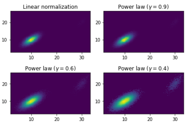
示例 1：

Python3

import matplotlib.pyplot as plt
import matplotlib.colors as mcolors
import numpy as np
from numpy.random import multivariate_normal
 
# data for reproducibility
data = np.vstack([
    multivariate_normal([10, 10],
                        [[3, 2],
                         [2, 3]],
                        size = 100000),
     
    multivariate_normal([30, 20],
                        [[2, 3],
                         [1, 3]],
                        size = 1000)
])
 
gammas_array = [0.9, 0.6, 0.4]
 
figure, axs = plt.subplots(nrows = 2,
                           ncols = 2)
 
axs[0, 0].set_title('Linear normalization')
axs[0, 0].hist2d(data[:, 0],
                 data[:, 1],
                 bins = 100)
 
for ax, gamma in zip(axs.flat[1:],
                     gammas_array):
     
    ax.set_title(r'Power law $(\gamma =% 1.1f)$' % gamma)
    ax.hist2d(data[:, 0],
              data[:, 1],
              bins = 100,
              norm = mcolors.PowerNorm(gamma))
 
figure.tight_layout()
 
plt.show()

输出：

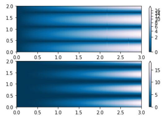
示例 2：

Python3

import numpy as np
import matplotlib.pyplot as plt
import matplotlib.colors as colors
 
max_N = 100
A, B = np.mgrid[-3:3:complex(0, max_N),
                -2:2:complex(0, max_N)]
 
 
# PowerNorm: using power-law
# trend in X
A, B = np.mgrid[0:3:complex(0, max_N),
                0:2:complex(0, max_N)]
 
X1 = (1 + np.sin(B * 10.)) * A**(2.)
 
figure, axes = plt.subplots(2, 1)
 
pcm = axes[0].pcolormesh(A, B, X1,
                         norm = colors.PowerNorm(gamma = 1./2.),
                         cmap ='PuBu_r')
 
figure.colorbar(pcm, ax = axes[0],
                extend ='max')
 
pcm = axes[1].pcolormesh(A, B, X1,
                         cmap ='PuBu_r')
 
figure.colorbar(pcm, ax = axes[1],
                extend ='max')
 
plt.show()

输出：