二次判别分析

线性判别分析

现在，让我们考虑由贝叶斯概率分布 P(Y=k | X=x) 表示的分类问题，LDA 通过尝试对给定预测变量类别（即 Y 的值）P(X =x| Y=k)：

$P(Y=k | X=x) = \frac{P(X=x | Y=k) P(Y=k)}{P(X=x)}$

$= \frac{P(X=x | Y=k) P(Y=k)}{\sum_{j=1}^{K} P(X=x | Y=j) P(Y=j)}$

在 LDA 中，我们假设 P(X | Y=k) 可以估计为多元正态分布，该分布由以下等式给出：

$f_k(x) = \frac{1}{(2\pi)^{p/2}|\mathbf\Sigma|^{1/2}} e^{-\frac{1}{2}(x-\mu_k)^T \mathbf{\Sigma}^{-1}(x-\mu_k)}$

在哪里， $\mu_k = mean\, of\, the\, examples\, of \, category\, k \\ \mathbf{\sum} = covariance \, (we\, assume\, common\, covariance\, for\, all\, categories)$

和 P(Y=k) =\pi_k。现在，我们尝试用以下假设写出上面的等式：

$P(Y=k | X=x) = \frac{\pi_k \frac{1}{(2\pi)^{p/2}|\mathbf\Sigma|^{1/2}} e^{-\frac{1}{2}(x-\mu_k)^T \mathbf{\Sigma}^{-1}(x-\mu_k)}}{\sum_{j=1}^{K} \frac{1}{(2\pi)^{p/2}|\mathbf\Sigma|^{1/2}} e^{-\frac{1}{2}(x-\mu_j)^T \mathbf{\Sigma}^{-1}(x-\mu_j)}}$

现在，我们对两边取对数并最大化方程，我们得到决策边界：

$\delta_k(x) = \log \pi_k - \frac{1}{2}\mu_k^T \Sigma^{-1}\mu_k + x^T \Sigma^{-1}\mu_k$

对于两个类，决策边界是 x 的线性函数，其中两个类的值相等，该线性函数为：

$\left\{x: \delta_k(x) = \delta_{\ell}(x) \right\}, 1 \leq j,\ell \leq K$

对于多类 (K>2)，我们需要估计 pK 均值、pK 方差、K 先验比例和$\binom{p}{2}K = \left ( \frac{p(p-1)}{2} \right )K$ .现在，我们更详细地讨论二次判别分析。

二次判别分析

二次判别分析与线性判别分析非常相似，只是我们放宽了所有类的均值和协方差相等的假设。因此，我们需要单独计算。

现在，对于每个 y 类，协方差矩阵由下式给出：

$\Sigma_y = \frac{1}{N_y-1} \sum_{y_i = y} (x_i - \mu_y)(x_i -\mu_y)^T$

通过添加以下项并求解（同时取对数 和 ）。二次判别函数由下式给出：

$\delta_k(x) = \log \pi_k - \frac{1}{2}\mu_k^T \mathbf{\Sigma}_k^{-1}\mu_k + x^T \mathbf{\Sigma}_k^{-1}\mu_k - \frac{1}{2}x^T \Sigma_k^{-1}x -\frac{1}{2}\log |\Sigma_k|$

执行

• 在这个实现中，我们将使用 R 和 MASS 库来绘制线性判别分析和二次判别分析的决策边界。为此，我们将使用 iris 数据集：

R

# import libraries
library(caret)
library(MASS)
library(tidyverse)
  
# Code to plot decision plot
decision_boundary = function(model, data,vars, resolution = 200,...) {
  class='Species'
  labels_var = data[,class]
  k = length(unique(labels_var))
  # For sepals
  if (vars == 'sepal'){
  data = data %>% select(Sepal.Length, Sepal.Width)
  }
  else{
  data = data %>% select(Petal.Length, Petal.Width)
  }
    
    
  # plot with color labels
  int_labels = as.integer(labels_var)
  plot(data, col = int_labels+1L, pch = int_labels+1L, ...)
    
  # make grid
  r = sapply(data, range, na.rm = TRUE)
  xs = seq(r[1,1], r[2,1], length.out = resolution)
  ys = seq(r[1,2], r[2,2], length.out = resolution)
  dfs = cbind(rep(xs, each=resolution), rep(ys, time = resolution))
    
  colnames(dfs) = colnames(r)
  dfs = as.data.frame(dfs)
    
  p = predict(model, dfs, type ='class' )
  p = as.factor(p$class)
  
    
  points(dfs, col = as.integer(p)+1L, pch = ".")
    
  mats = matrix(as.integer(p), nrow = resolution, byrow = TRUE)
  contour(xs, ys, mats, add = TRUE, lwd = 2, levels = (1:(k-1))+.5)
    
  invisible(mats)
}
  
par(mfrow=c(2,2))
# run the linear disciminant analysis and plot the decision boundary with Sepals variable
model = lda(Species ~ Sepal.Length + Sepal.Width, data=iris)
lda_sepals = decision_boundary(model, iris, vars= 'sepal' , main = "LDA_Sepals")
  
# run the quadratic disciminant analysis and plot the decision boundary with Sepals variable
model_qda = qda(Species ~ Sepal.Length + Sepal.Width, data=iris)
qda_sepals = decision_boundary(model_qda, iris, vars= 'sepal', main = "QDA_Sepals")
  
# run the linear disciminant analysis and plot the decision boundary with Petals variable
model = lda(Species ~ Petal.Length + Petal.Width, data=iris)
lda_petal =decision_boundary(model, iris, vars='petal', main = "LDA_petals")
  
# run the quadratic disciminant analysis and plot the decision boundary with Petals variable
model_qda = qda(Species ~ Petal.Length + Petal.Width, data=iris)
qda_petal =decision_boundary(model_qda, iris, vars='petal', main = "QDA_petals")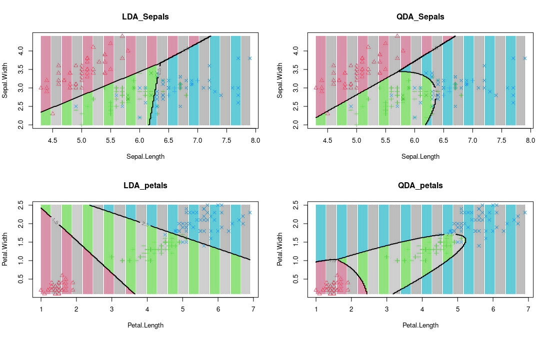

LDA 和 QDA 可视化

参考：

• 斯坦福统计笔记
• 哈佛关于 LDA 的幻灯片